How to Get Current Stock Price of India in Excel: 3 Ways

Download Practice Workbook

Download this practice workbook to exercise while you are reading this article.

Current Stock Price India.xlsx

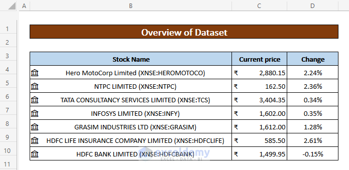
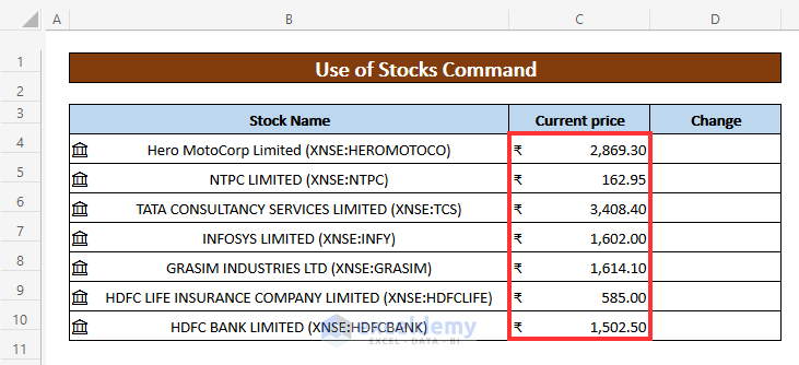
Let’s say we have a dataset containing several Indian stock company names, current prices, and the percentage of change in columns B, C, and D, respectively. Here’s how to get the current stock price of the Indian stock market.

Method 1 – Use STOCKHISTORY Function to Get Current Stock Price of India

Step 1:

Apply the TODAY function in cell D15 to get today’s date:

=TODAY()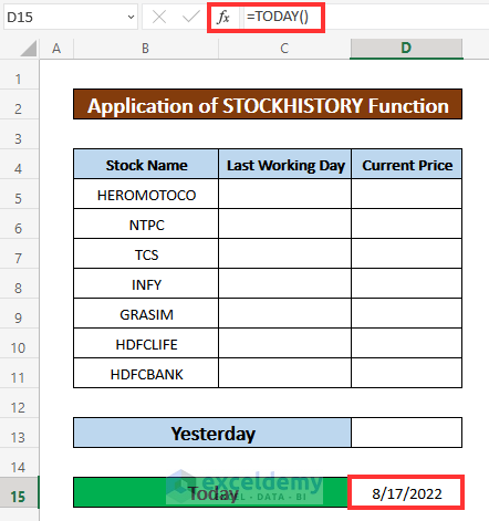

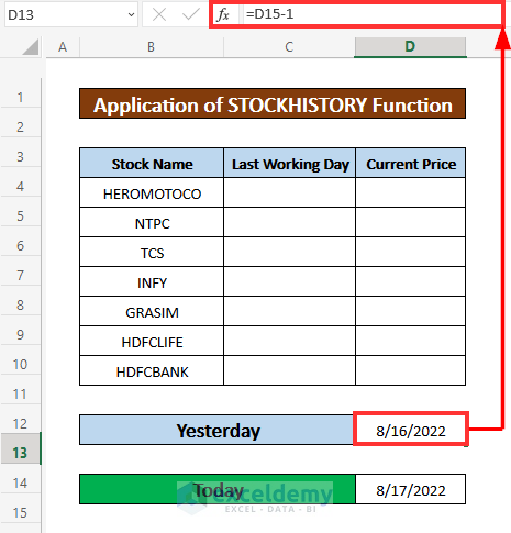
Use the following formula in cell D13 to get the previous date:

=D15-1

Press Enter to get the yesterday’s date in the cell.

Step 2:

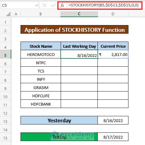
Select cell C5 and write down the STOCKHISTORY Function in that cell:

=STOCKHISTORY(B5,$D$13,$D$15,0,0)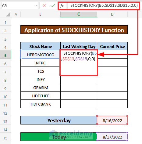

Press ENTER on your keyboard, and you will get the current price of that corresponding date. The current price at time of writing is ₹ 2,817.00.

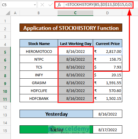
AutoFill the STOCKHISTORY function in the rest of the cells in column D to get the current price of the Indian stock market.

Method 2 – Apply Stock Command to Get Current Stock Price of India

Steps:

Select the entire range of cells B5:B11.
Go to the Data ribbon and select Stocks:

Data → Data Types → Stocks

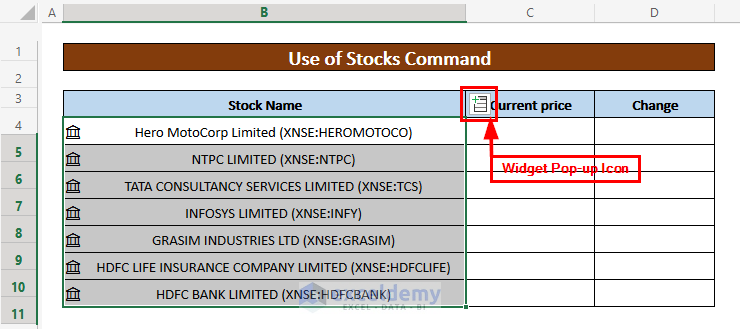
Excell will search for the company’s full name and stock market abbreviation and fill it in. Next to the names, you will see a small widget pop-up icon appear at the right corner.

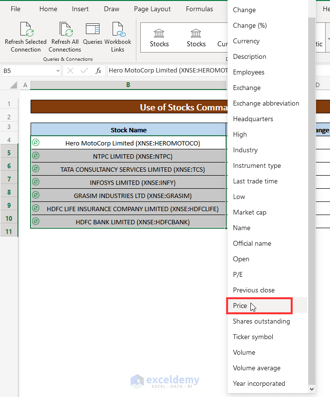
If you click on it, you will get several fields listed there. We are going to add only the Price and Change(%) fields.
Click on the widget pop-up icon, scroll down, and select the Price option.

You will see the Price of all the companies added to cells C5:C11.

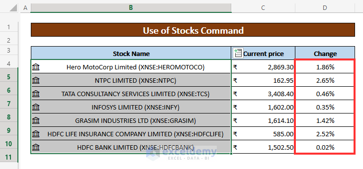
Repeat to add the Change(%) field in column D.

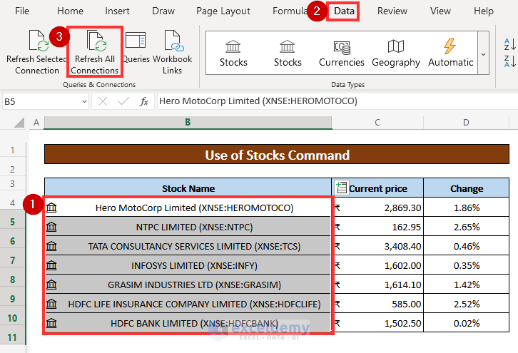
In the Data ribbon, go to Queries & Connections and select Refresh All Connections.

Method 3 – Using Power Query to Get Current Stock Price of India

Steps:

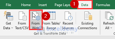
From your Data ribbon, go to Get & Transform Data, then select From Web.

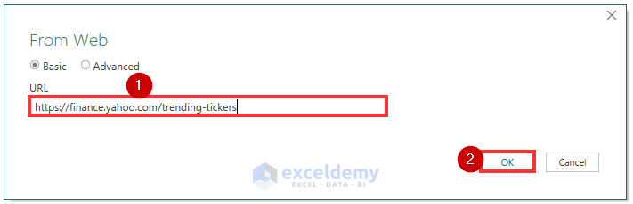
A small dialog box titled From Web will appear.
Choose the Basic option and paste the website link into the empty box. We are pasting a link from Yahoo Finance.
Click on OK and wait for a bit.

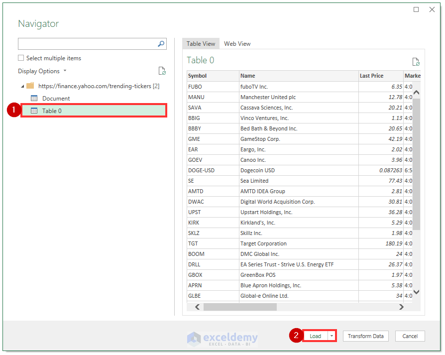
The Navigator window should appear in front of you.
Select Table 0 and click on the Load. The panel will also show you a visual representation of that dataset.

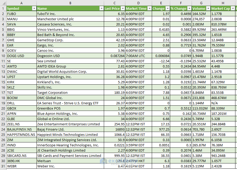
The current stock price list will be in your Excel spreadsheet. Format the key columns to get a better outlook of your dataset.

Things to Remember

➜ You can perform Method 1 and Method 2 in Microsoft Office 365 only. You can use Power Query in Excel 365 and any other version.

➜ If Excel can’t find a value (such as the name of a company), it will show the #N/A! error.

➜ #DIV/0! error happens when a value is divided by zero(0) or the cell reference is blank.

How to Import Stock Prices into Excel from Google Finance

<< Go Back to Stocks In Excel| Excel for Finance | Learn Excel

Get FREE Advanced Excel Exercises with Solutions!

Sub FetchDataFromAllPagesOfAWeb() Dim pageNumber As Integer Dim urlBase As String Dim queryName As String Dim queryFormula As String Dim ws As Worksheet Dim startCell As Range Dim masterSheet As Worksheet Application.DisplayAlerts = False Application.ScreenUpdating = False Set masterSheet = ThisWorkbook.Sheets.Add masterSheet.Name = "Master Sheet" Call deleteQueriesAndConnections urlBase = "https://www.screener.in/screens/16162/all-stocks/?sort=name&order=asc&page=" pageNumber = 1 Do While pageNumber <= 69 queryName = "Table_" & pageNumber - 1 queryFormula = "let" & Chr(13) & Chr(10) & _ " Source = Web.Page(Web.Contents(""" & urlBase & pageNumber & """))," & Chr(13) & Chr(10) & _ " Data0 = Source{0}[Data]," & Chr(13) & Chr(10) & _ " #""Changed Type"" = Table.TransformColumnTypes(Data0,{{""S.No."", Int64.Type}, {""Name"", type text}, {""CMP Rs."", type number}, {""P/E"", type number}, {""Mar Cap Rs.Cr."", type number}, {""Div Yld %"", type number}, {""NP Qtr Rs.Cr."", type number}, {""Qtr Profit Var %"", type number}, {""Sales Qtr Rs.Cr."", type number}, {""Qtr Sales Var %"", type number}, {""ROCE %"", type number}, {""Debt / Eq"", type number}, {""B.V. Rs."", type number}})" & Chr(13) & Chr(10) & _ "in" & Chr(13) & Chr(10) & _ " #""Changed Type""" Set ws = ThisWorkbook.Sheets.Add ws.Name = "Page_" & pageNumber ActiveWorkbook.Queries.Add Name:=queryName, Formula:=queryFormula With ws.ListObjects.Add(SourceType:=0, Source:= _ "OLEDB;Provider=Microsoft.Mashup.OleDb.1;Data Source=$Workbook$;Location=""" & queryName & """;Extended Properties=""""" _ , Destination:=ws.Cells(2, 1)).QueryTable .CommandType = xlCmdSql .CommandText = Array("SELECT * FROM [" & queryName & "]") .RowNumbers = False .FillAdjacentFormulas = False .PreserveFormatting = True .RefreshOnFileOpen = False .BackgroundQuery = True .RefreshStyle = xlInsertDeleteCells .SavePassword = False .SaveData = True .AdjustColumnWidth = True .RefreshPeriod = 0 .PreserveColumnInfo = True .ListObject.DisplayName = queryName .Refresh BackgroundQuery:=False End With ws.UsedRange.Copy Destination:=masterSheet.Cells(masterSheet.Cells(Rows.Count, 1).End(xlUp).Row + 1, 1) 'ThisWorkbook.Queries(queryName).Delete pageNumber = pageNumber + 1 Loop Dim wsToDelete As Worksheet For Each wsToDelete In ThisWorkbook.Sheets If wsToDelete.Name <> "Master Sheet" Then wsToDelete.Delete End If Next wsToDelete Application.ScreenUpdating = True Application.DisplayAlerts = True End Sub Sub deleteQueriesAndConnections() Dim QueriesAndConnections As Object For Each QueriesAndConnections In ThisWorkbook.Queries QueriesAndConnections.Delete Next End Sub

10 Comments

amit Aug 22, 2022 at 9:43 PM

Update function work work in Google sheets itself or have to go to linked excell sheet in window
- Reply
  Sabrina Ayon Aug 24, 2022 at 2:19 PM
  
  Hello, AMIT!
  I’m really sorry to say that the STOCKHISTORY function won’t work in Google Sheet as google sheet has limited functions to perform but the TODAY function will work adequately. You need to work on an Excel sheet.
vadakkus Oct 3, 2022 at 12:32 PM

Hi sir, Stocks option is only showing NASDAQ index. how do I get Indian scrips there?
Md. Abdur Rahim Rasel Oct 4, 2022 at 1:40 PM

Hello VADAKKUS!
To get the Stocks of the Indian Index instead of the NASDAQ Index, please use the below link in Method 3. The link is: https://www.moneycontrol.com/markets/indian-indices/
Thank you for your comment.
Regards
Md. Abdur Rahim Rasel (Exceldemy Team)
RAMAN Feb 24, 2023 at 11:15 PM

I AM NOT GETTING STOCK OPTION IN DATA TYPE IN MY EXCEL EVEN AFTER HAVING LATEST VERSION OF EXCEL AND MICROSOFT OFFICE . CAN YOU PLEASE HELP ME WITH THAT ?
- Reply
  Adnan Masruf Feb 27, 2023 at 1:50 PM
  
  Dear Raman,
  1. First, make sure you are using MS Office 365 as they are only available in that version.
  2. Secondly, make sure you are logged into your MS Excel account.
  3. Thirdly, make sure to have the English, French, German, Italian, Spanish, or Portuguese editing language added to Office Language Preferences.
  If these do not work then,
  -Go to File > Options > Trust Center > Trust center Settings > External Content > Security settings for “Linked data types” > Activate “Enable all Linked Data Types”
  or
  – Go to Options>Customize Ribbon> All Commands
  – Then, choose the Datatype Command
  -Add the command to a “New Group”
  -Finally, restart your Excel Application.
  
  *Also, make sure to keep your internet connection ON; as this data type is linked datatype.
  *You should also see if this datatype is available in your geopolitical locaton.
Bala Apr 16, 2023 at 10:59 PM

Hi Sir,
Is there a way to get the current Mutual Fund NAVs in an excel sheet which will be automatically updated every end of the day ?
Kindly share a sample excel sheet for Mutual funds.

Best regards
Bala
- Reply
  Akib Bin Rashid Apr 17, 2023 at 12:43 PM
  
  Hi BALA Sir
  Thank you for your comment.
  To get the current mutual fund NAVs, you can use the following link:
  https://scripbox.com/mutual-fund/latest-nav
  You can get the latest NAVs using PowerQuery (method 3 in this article).
  You will need to activate the “link to data” option to get the automatic update.
  I think it should work this way. Please let us inform if you face any issues.
  Thank you

AJK Nov 1, 2023 at 12:08 PM

Hi Rasel,

Thank you for the comprehensive explanation.
I am using Excel in MS Office Professional Plus 2019 to track my stocks. As I understand, I can use only Power Query to link my excel sheet to the Stock Price display. Have found that https://www.screener.in/screens/16162/all-stocks/?sort=name&order=asc is a better option than the NSE or BSE sites since all Indian scripts are displayed there on a single page.
However in Table 0, only 25 scripts are displayed, and am unable to display all the scripts reuqired even after repeatedly refreshing the Queries and Connections tab. Is there any workaround for this?

Lutfor Rahman Shimanto Nov 2, 2023 at 12:13 PM

Hello AJK

Thanks for sharing this exciting issue with us. The mentioned site arranges the required information on many pages. When I went through, there were 69 pages (25 records are displayed on each page). However, the page numbers will change over time. You wanted to use the PowerQuery and fetch all the information into a single sheet.

I am delighted to inform you that I have developed an Excel VBA Sub-procedure to fulfil your requirements. Thanks to MD. ABDUR RAHIM RASEL. I developed such an Excel VBA Sub-procedure by considering the idea he had given in the previous comment.

Excel VBA Sub-procedure:

OUTPUT:
Output of running Excel VBA code

Things to Remember:

1. Add a new sheet and delete the Master Sheet before running the Excel VBA Code.

2. At the end of the code execution, the code will delete all sheets except for the Master Sheet.

Limitations: The code will take 10 to 15 minutes to fetch data from that site. It will depend on the capacity of your computer and internet connection.

I am attaching the solution workbook for better understanding. Good luck!
Download Solution Workbook

Regards
Lutfor Rahman Shimanto

How to Get Current Stock Price of India in Excel: 3 Ways

Method 1 – Use STOCKHISTORY Function to Get Current Stock Price of India

Method 2 – Apply Stock Command to Get Current Stock Price of India

Method 3 – Using Power Query to Get Current Stock Price of India

Things to Remember

Related Article

Leave a reply Cancel reply