In this article, we will demonstrate some of the most commonly used methods of calculating safety stock in Excel, from the simple arithmetic way to some non-conventional but precise methods, and how to calculate reorder points from calculated safety stock.
Download Practice Workbook
What is Safety Stock?
Safety stock, also known as buffer stock, is used in inventory and supply chain management, and indicates the additional stock that a business keeps on hand as a security against the change in demand and supply.
Safety Stock Formula
The most used formulas to determine safety stock are:
- Basic Formula of Safety Stock: Average Sales * Stock available
- Safety Stock Based on Average-Max Method: (Max. lead time*Max. sales in a day) – (Avg. lead time*Avg. Sales in a day)
- Safety Stock Using Kings Method: Coefficient service (Z) * √(Average Lead Time * (Demand S.D)2 + (Average Sales * Lead Time S.D)2)
Calculating Safety Stock in Excel
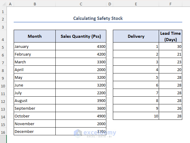
We will be using the following dataset to illustrate our methods. The dataset contains a shop’s sales quantity per month and the delivery lead time.
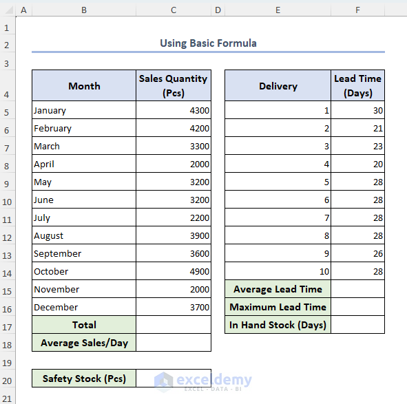
Method 1 – Using the Basic Formula
Let’s start by calculating the safety stock in an old-fashioned way. For this method, we need to assume the number of safety days for the safety stock.
STEPS:
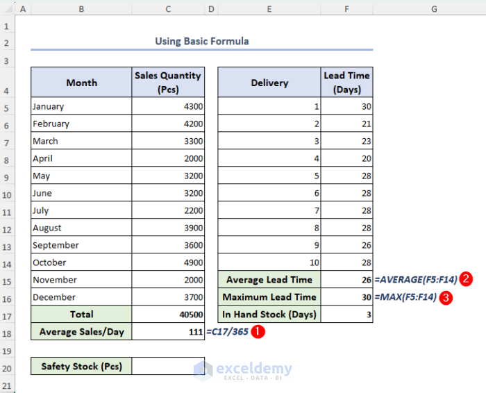
- Modify our dataset as follows:
First we calculate the total quantity sold using Excel SUM function.
- Select cell C17, enter the formula below, and press Enter:
=SUM(C5:C16)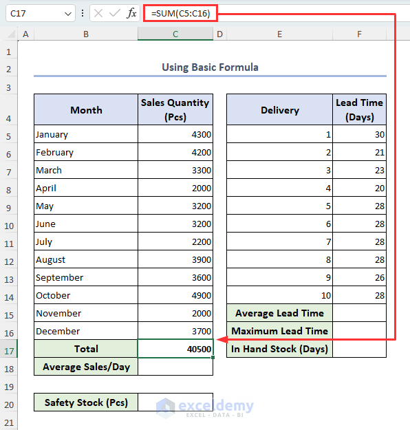
Now we calculate the values of average sales per day, average lead time, and maximum lead time.
- Enter the formulas below in cells C18, F15, F16 respectively:
=C17/365=AVERAGE(F5:F14)=MAX(F5:F14)Let’s assume we have 3 days of in-hand stock in our hands.
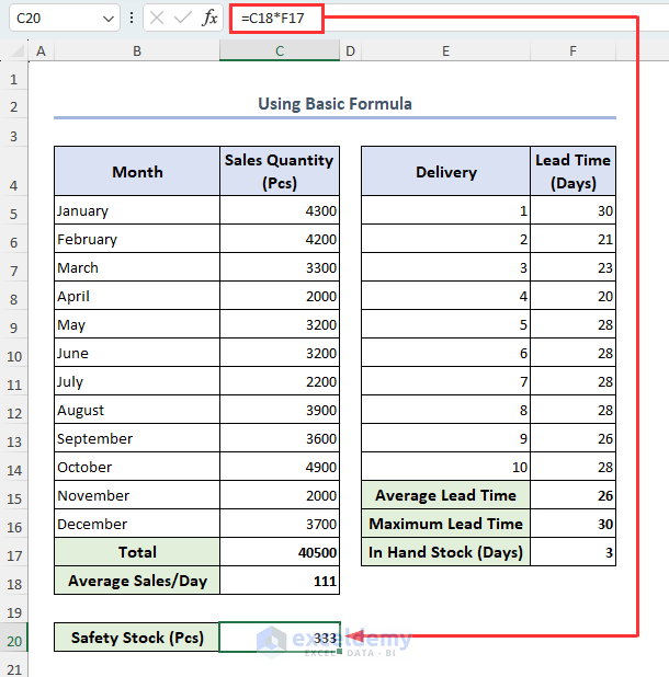
- Select cell F17 and type 3.
- Select cell C20, insert the formula below, and hit Enter:
=C18*F17The formula for this method:
The value of Average Sales is returned in cell C18 and the value of Stock Available is in cell F17.
Method 2 – Using the Average-Max Method
The previous approach offered a foundational understanding of safety stock which is not recommended for usage in real-life situations. We suggest using this approach as opposed to that outdated method. If we consider the worst case for supply and demand fluctuation, this approach to calculate safety stock in Excel is appropriate. Here, Excel’s AVERAGE and MAX formulas have been combined to derive the safety stock.
STEPS:
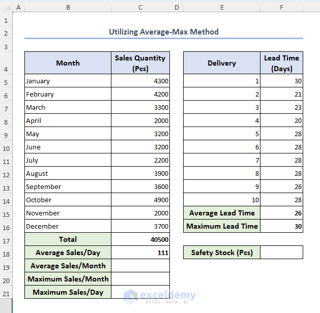
- Modify the previous dataset as below. We use the total sales, average sales per day, average lead time, and maximum lead time that we calculated in Method 1 above here too.
- To calculate average sales per month, maximum sales per month, and maximum sales per day, simply select cells C19, C20 and C21 and insert the following formulas respectively:
=C17/12=MAX(C5:C16)=C20/30.5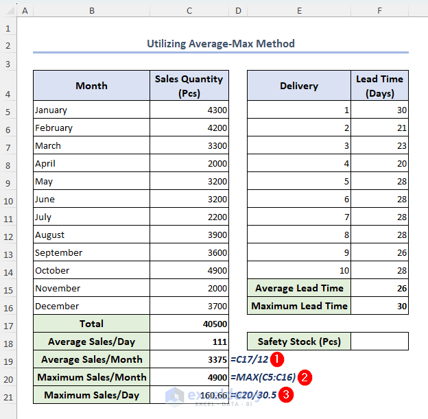
The formula for safety stock for the Average Max method is:
The value of lead time is in cell F16, the value of Max. sales in a day is in cell C21, the value of Avg. lead time is in cell F15 and the value of Avg. Sales in a day is in cell C18.
- Select cell F18, enter the formula below, and hit Enter:
=(F16*C21)-(F15*C18)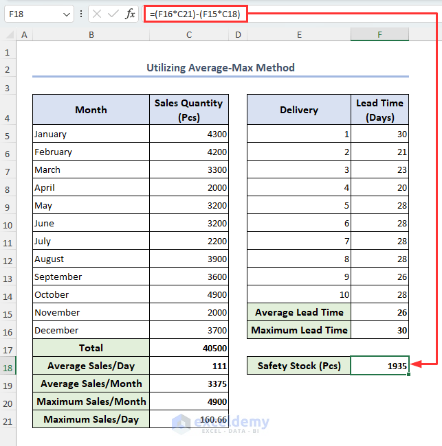
The safety stock returns in cell F18.
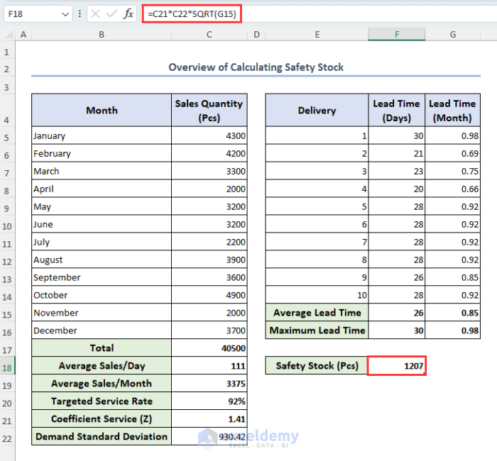
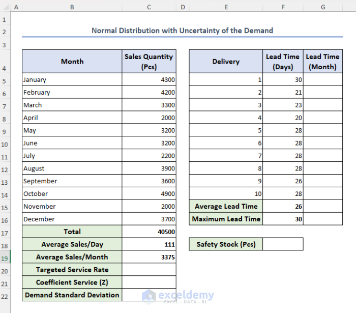
Method 3 – Normal Distribution with Uncertainty of Demand
This method is appropriate if you want to manage safety stock using a tolerance of your choosing. We will use normal distribution if we have uncertainty of demand. Compared to the previous method, we use time units in months, for which we add a new column.
STEPS:
- Modify the previous dataset as follows:
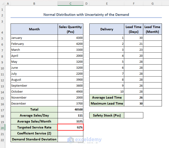
Let’s assume our targeted service rate is 92%.
- Select cell C20 and type 92%.
We can determine the value of coefficient service (Z) using Excel’s built-in NORMSINV function and the value of demand standard deviation using Excel STDEV function.
- Select cells C21 and C22 and insert the following formulas respectively:
=NORMSINV(C20)=STDEV(C5:C16)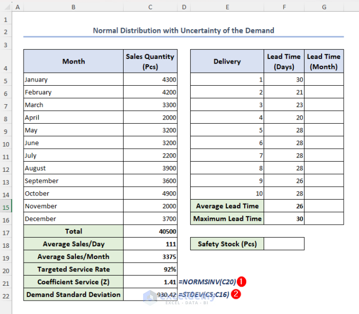
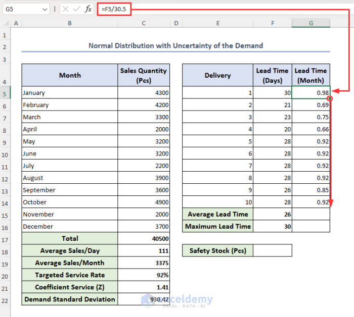
- To calculate monthly lead time, select cell G5, insert the formula below, and press Enter:
=F5/30.5- Use the Fill handle icon to drag the formula down to the rest of the cells in the column.
Now, we will calculate the monthly average lead time and monthly maximum lead time.
- In cells G15 and G16, enter the formulas below respectively:
=AVERAGE(G5:G14)=MAX(G5:G14)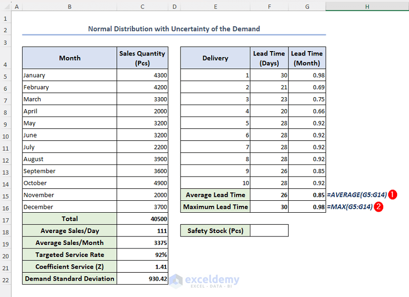
Safety Stock for Normal Distribution with Uncertainty of the Demand = Coefficient service (Z) * Demand Standard Deviation * √ Monthly Average Lead Time
- In cell F18, enter the below formula and press Enter:
=C21*C22*SQRT(G15)Here, cell C21 carries the value of Z, cell C22 represents the value of demand standard deviation and cell G15 has the value of monthly average lead time.
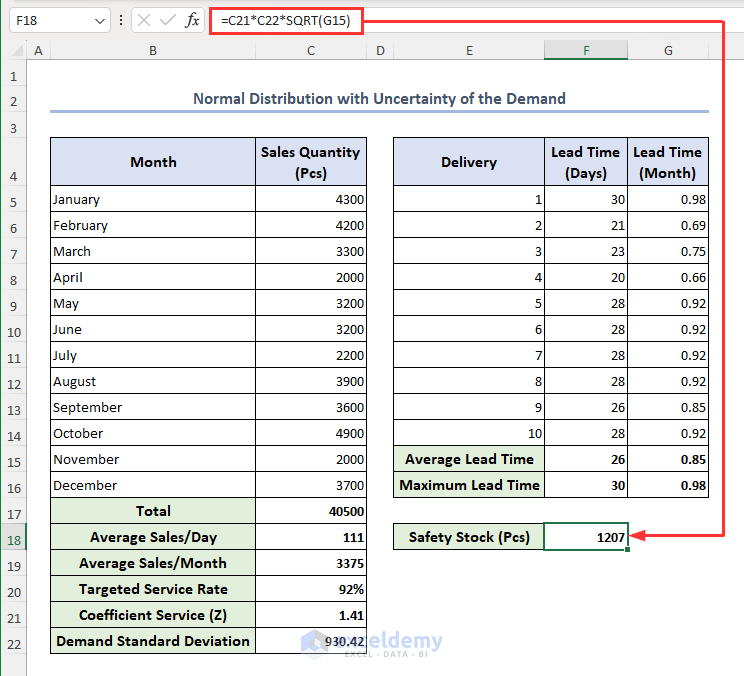
The value of safety stock is returned in cell F18.
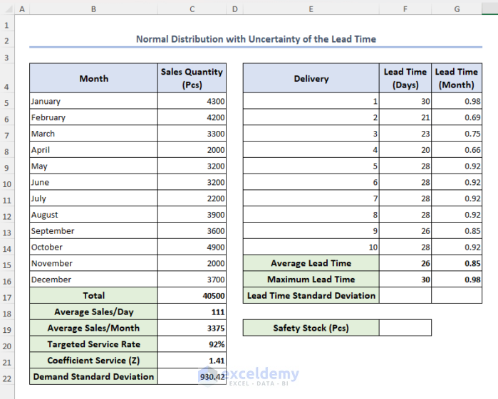
Method 4 – Normal Distribution with Uncertainty of the Lead Time
Now we consider uncertainty of lead time only, so we need to determine the lead time standard deviation.
STEPS:
- Modify the previous dataset as follows:
- To calculate day-wise lead time standard deviation, select cell F17 and insert the formula below, then press Enter:
=STDEV(F5:F14)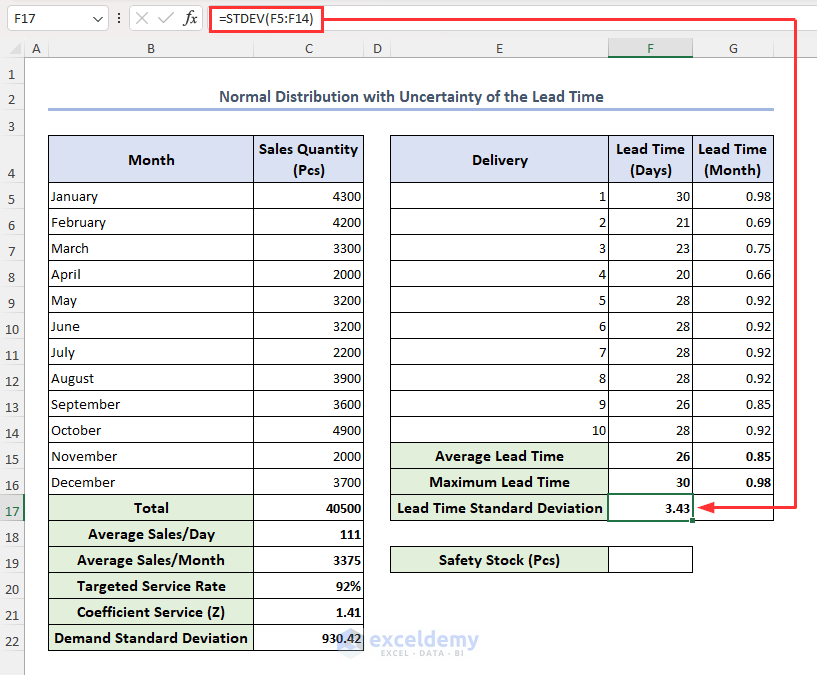
- To calculate month-wise lead time standard deviation, enter the following formula in cell G17 then press Enter:
=STDEV(G5:G14)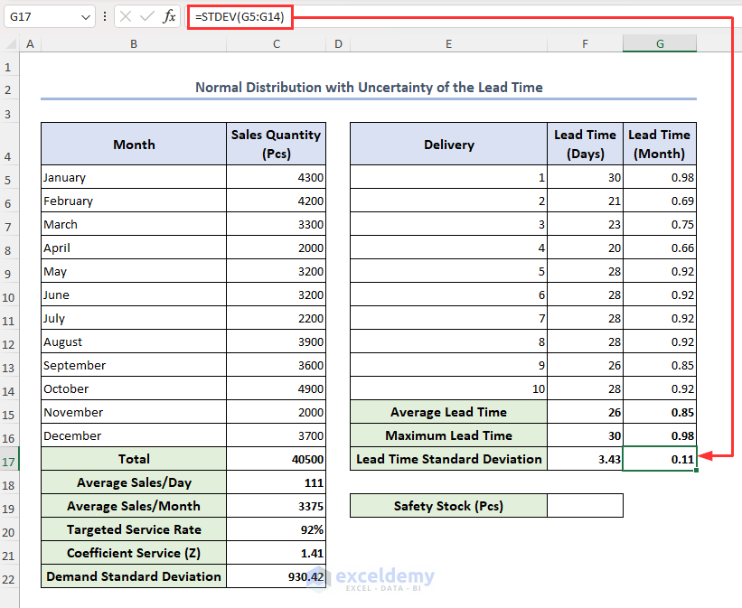
Safety Stock for Normal Distribution with Uncertainty of the Lead Time = Coefficient Service (Z) * Average Sales per Month * Month wise Lead time standard deviation
- Enter the formula below in cell F19 and press Enter:
=C21*C19*G17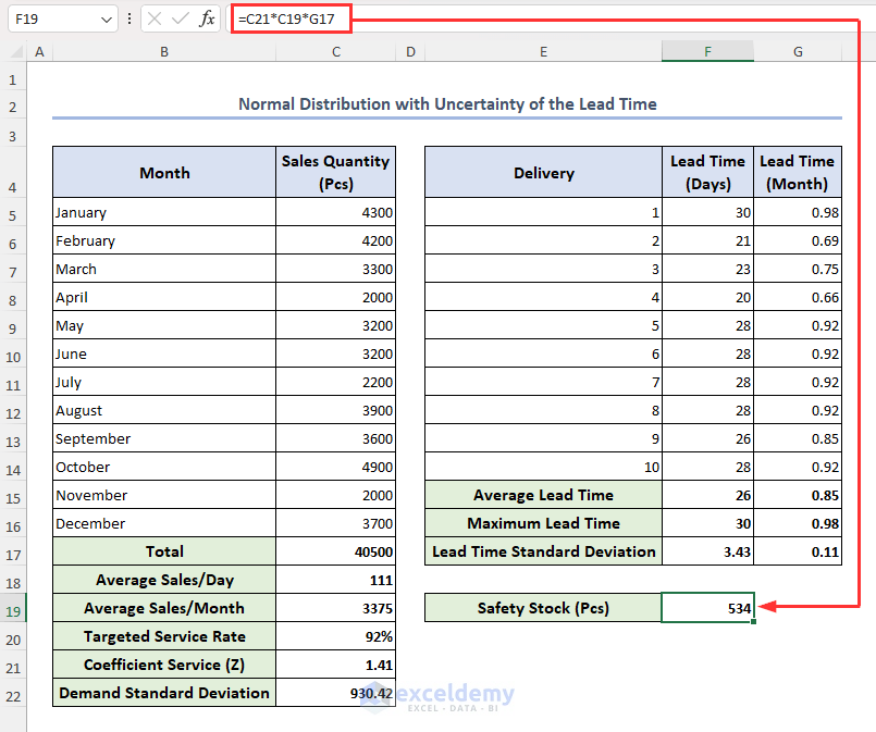
The value for safety stock is returned in cell F19.
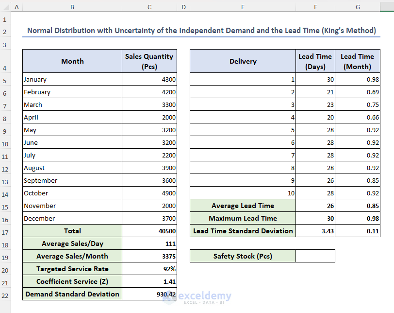
Method 5 – Normal Distribution with Uncertainty of the Independent Demand and the Lead Time (King’s Method)
In this method, we consider both lead time and demand uncertainty, assuming both as independent. This method is also known as King’s Method and is the most accepted method to calculate safety stock in Excel. A change in lead time doesn’t affect the demand in this method.
Our formula based on King’s Method is:
- In the following dataset, cells C21, G15, C22, C19 and G17 have the values of Coefficient service (Z), Monthly Average Lead Time, Demand S.D, Average Sales per Month, and Lead Time S.D respectively.
- Select cell F19, enter the formula below and press Enter:
=C21*SQRT((G15*C22^2)+(C19*G17)^2)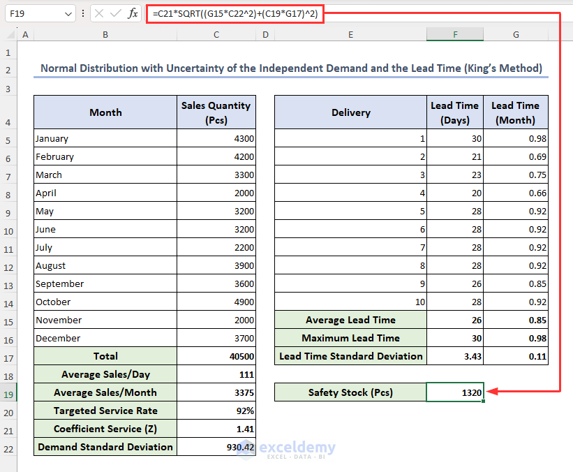
This returns you the value of safety stock in cell F19.
Method 6 – Normal Distribution with Uncertainty of the Dependent Demand and the Lead Time
In this method, we consider both lead time and demand uncertainty, assuming both as dependent. A change in lead time affects the demand.
Formula for this method:
- Select cell F19, enter the formula below, and hit Enter:
=C21*C22*SQRT(G15)+C21*C19*G17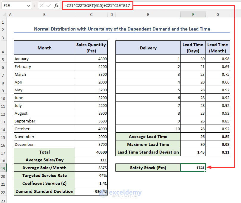
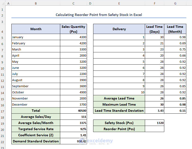
How to Calculate Reorder Point from Safety Stock in Excel
A company’s reorder point is the amount of inventory it must have on hand before placing a new order. It is calculated based on the expected demand, lead time, and the safety stock required for variability in demand and supply.
The formula for reorder point is:
From King’s method, our dataset is as below.
Now we will calculate the reorder point from these data.
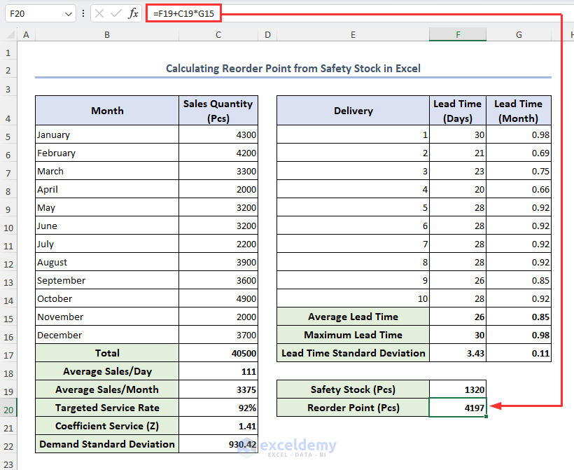
STEPS:
- Select cell F20, enter the formula below then press Enter:
=F19+C19*G15The value of reorder point will return in cell F20.
Why is Safety Stock Necessary?
Safety stock is essential because it serves as a backup supply to stop product shortages. It assists in managing unexpected increases in demand, delays in receiving new stock, and mistakes in estimating the amount of inventory required. Businesses may meet client requests even in disruptive or difficult circumstances because of safety stock.
Downsides of Safety Stock
- Extra inventory kept on hand as Safety Stock may use up available funds and drive up storage expenses.
- Safety Stock can become obsolete if it is not used, causing waste and financial losses.
- The amount of Safety Stock that may be held may be limited by a lack of storage capacity, causing shortages during unexpected demand increases.
- Effective inventory management procedures for handling Safety Stock can be difficult and time-consuming to implement.
Frequently Asked Questions
1. How do you calculate Z in safety stock?
Z represents coefficient service, and can be calculated in Excel using its built-in NORMSINV function. Let’s assume your targeted service rate’s value is in cell A1. Pick an empty cell and enter this formula:
=NORMSINV(A1)This will return the value of Z.
2. What is safety stock level?
Safety stock or safety stock level or buffer stock, all have similar meanings. The amount of additional inventory a business keeps on hand to guard against unexpected changes in demand or supply is known as the safety stock level.
3. What is lead time demand?
The term lead time demand describes the total amount of demand for a good or service while the inventory is being refilled. It also includes the demand that arises after an order has been placed while a new supply is being delivered.
Get FREE Advanced Excel Exercises with Solutions!

