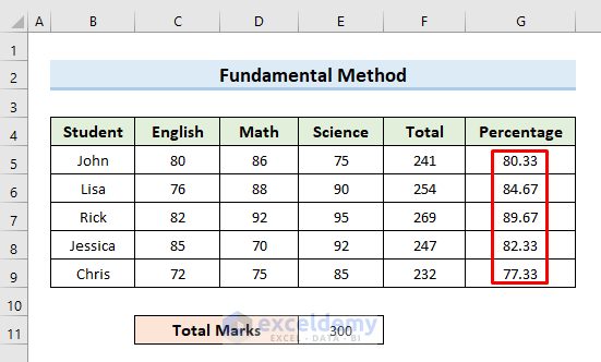
Method 1 – Fundamental Percentage Formula in Excel for a Marksheet
If we want to determine what percentage of A is B we will use the following formula.

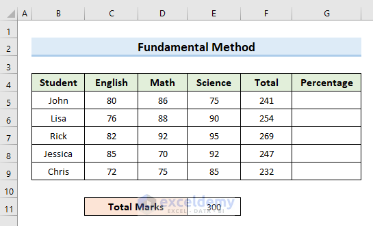
We have marks for 3 subjects for five students and their total obtained marks. Here, the total mark for 3 subjects is 300. We will calculate what percentage of total marks each student gets.
Steps:
- Select cell G5.
- Insert the following formula in that cell:
=(F5/300)*100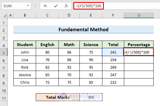
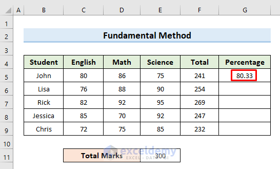
- Press Enter.
- Select cell G5 again.
- Move the mouse cursor to the bottom right corner of the selected cell so that it turns into a plus (+) sign like the following image.
- Click on the plus(+) sign and drag the Fill Handle down to cell C9 to copy the formula of cell G5 in other cells. You can also double-click on the plus (+) sign to get the same result.
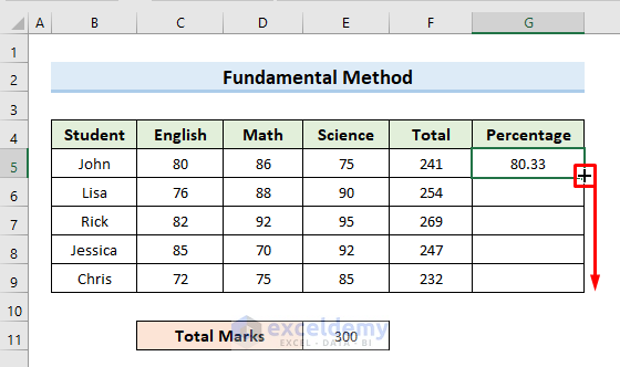
- This copies the formula of cell G5 to the other cells.
Read More: Make an Excel Spreadsheet Automatically Calculate Percentage
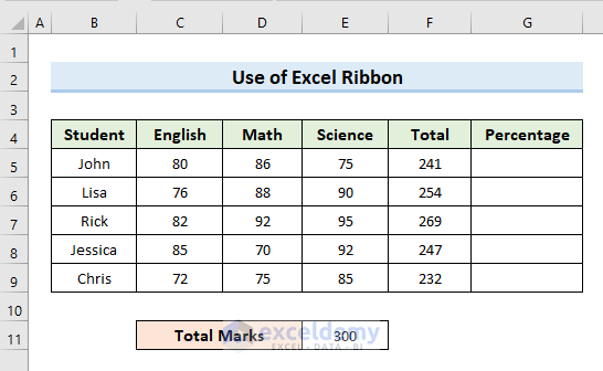
Method 2 – Apply a Percentage Formula from Excel Ribbon
We will calculate the percentage of our previous dataset again.
Steps:
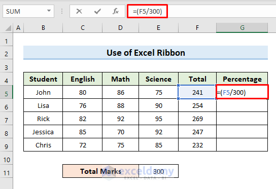
- Select cell G5.
- Insert the following formula in that cell:
=(F5/300)- We have not multiplied the value by 100 here like the previous example.
- Press Enter. This returns the value in decimals.
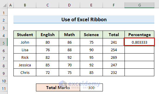
- Go to the Home tab.
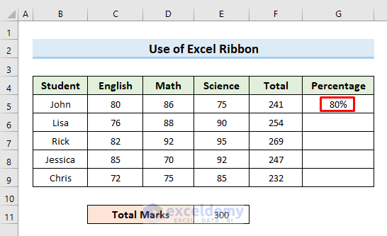
- Select the option Percent Style (%) or press Ctrl + Shift + % after selecting the cell G5.
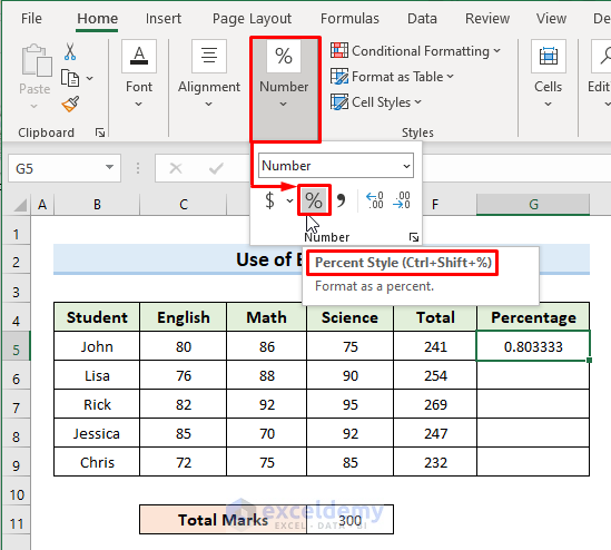
- This converts the decimal value into a percentage.
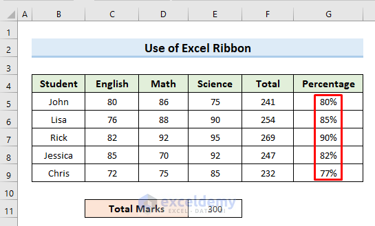
- Drag the Fill Handle tool from C5 to cell G9.
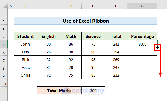
- This returns all the values in percentages.
Related Content: How to Apply Percentage Formula for Multiple Cells in Excel
Method 3 – Extract a Particular Value Using Percentage Formula in Excel
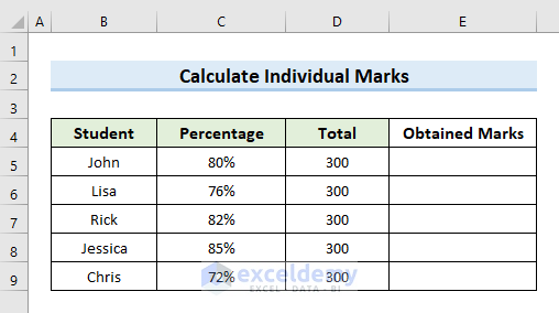
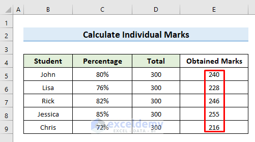
Case 3.1 – Evaluate Individual Marks by Total and Percentage
In the following dataset, we have the total marks and percentages gained by all students. We will calculate the Obtained Marks for each student.
Steps:
- Select cell E5.
- Insert the following formula in that cell:
=D5*C5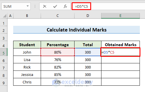
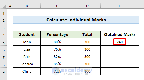
- Hit Enter.
- Drag the Fill Handle tool to cell E9.
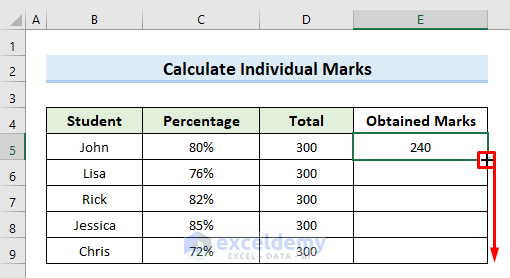
- This returns the marks for all students in cells (G5:G9).
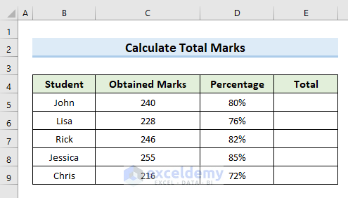
Case 3.2 – Use Individual Marks and a Percentage to Evaluate Total Marks
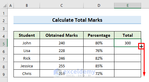
We have the value of Obtained Marks and Percentage in our following dataset. We will calculate the total marks by using these two values.
Steps:
- Select cell E5.
- Insert the following formula in that cell:
=C5/D5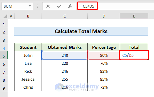
- Press Enter.
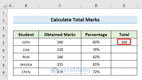
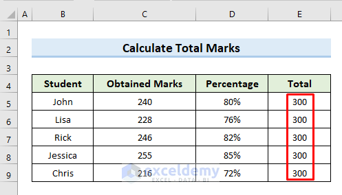
- Drag the Fill Handle tool to cell E9.
- This returns the value of total marks in cells (E5:E9).
Read More: How to Calculate Total Percentage in Excel
Method 4 – Use Percentage Formulas in Excel to Modify Existing Marks by a Percentage
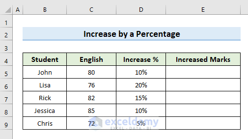
Case 4.1 – Increase Marks by a Percentage
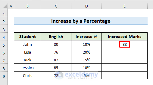
We have the following dataset, which contains the obtained marks for six students in the subject of English. We will increase the marks of each student by different percentages.
Steps:
- Select cell E5.
- Insert the following formula in that cell:
=C5*(1+D5)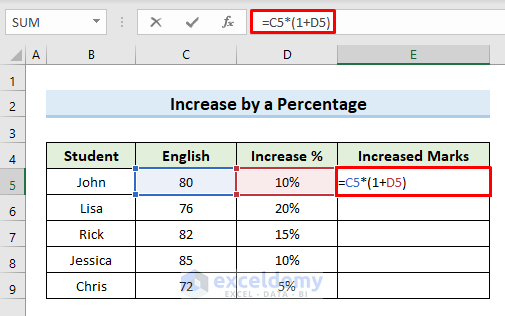
- Hit Enter. We get the increased value in cell E5.
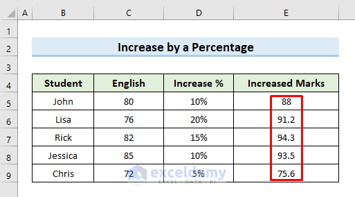
- Drag the Fill Handle tool to cell E9.
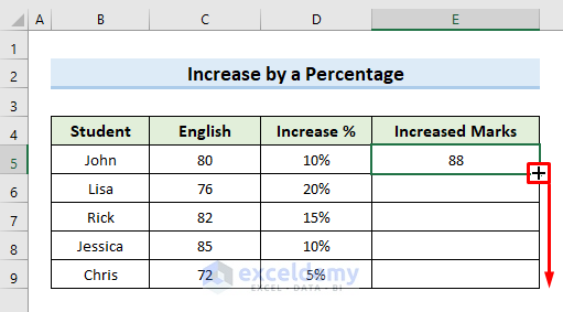
- This fills in the cells (E5:E9).
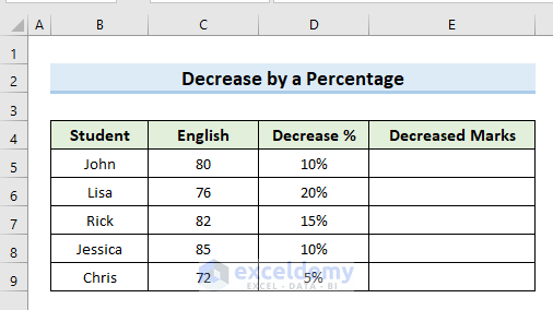
Case 4.2 – Decrease Marks by a Percentage
We will decrease the value of obtained marks by a specific percentage.
Steps:
- Select cell E5.
- Insert the following formula in that cell:
=C5*(1-D5)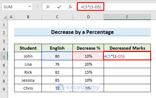
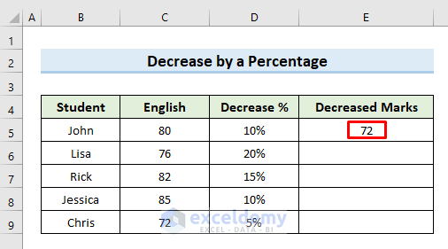
- Hit Enter.
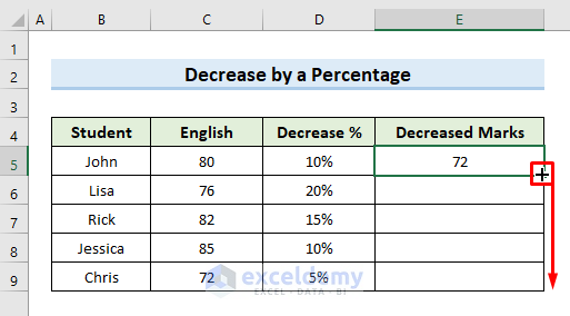
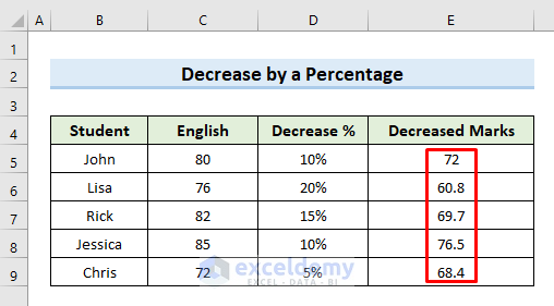
- Drag the Fill Handle tool to cell E9.
- We can see the decreased marks for all students in cells (E5:E9).
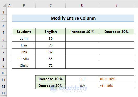
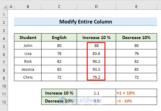
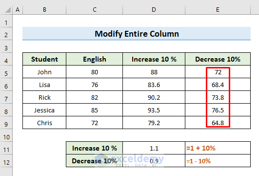
Method 5 – Modify the Entire Column of a Marksheet With a Percentage Formula in Excel
In the following dataset, we have a mark sheet of six students containing their marks in English. We’ll increase and decrease the marks of all students by 10%.
Steps:
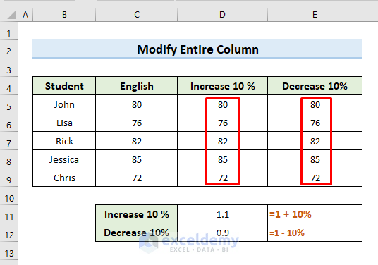
- Copy the same value of marks in the columns “Increased 10%” and “Decreased 10%”.
- Increasing by 10% means multiplying by 1.1 and decreasing by 10% means a multiplier of 0.9.
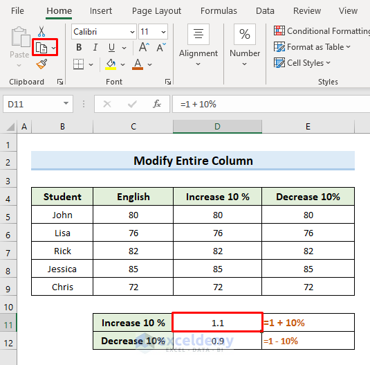
- Select cell D11.
- Click on the Copy from ribbon or press Ctrl + C.
- Select the cells (D5:D9) and go to Paste Special.
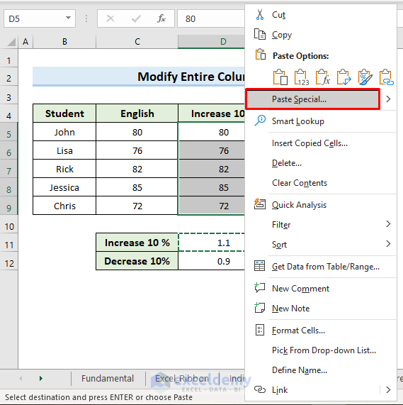
- A new dialogue box will appear.
- Check the option “Multiply” from that box.
- Press OK.

- This increases all the values of cells (D5:D9) by 10%.
- Follow the same process with the cell D12 and the range (E5:E9).
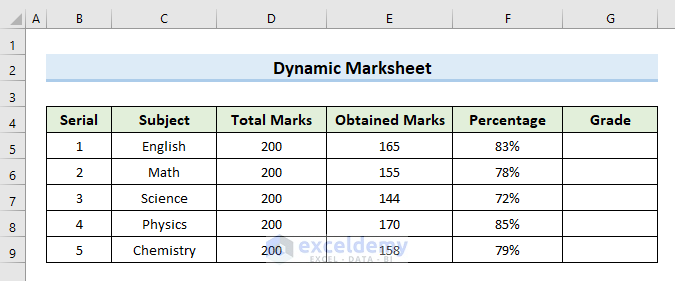
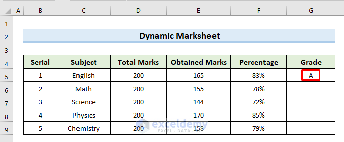
Method 6 – Create a Dynamic Marksheet in Excel
We will create a dynamic mark sheet by using the percentage formula.
Steps:
- Select cell G5 and insert the following formula:
=IF(F5<40%,"F",IF(F5<60%,"C",IF(F5<80%,"B","A")))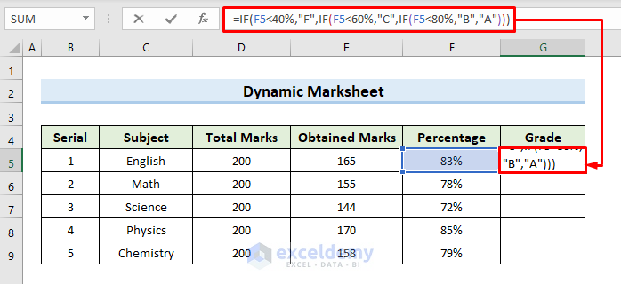
- Hit Enter.
- Drag the Fill Handle tool to cell G9.
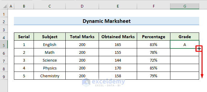
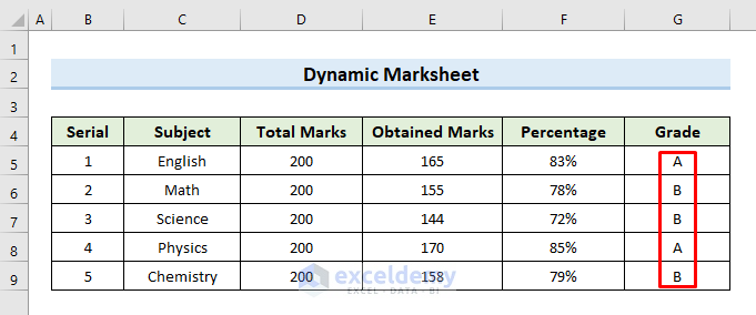
- We can see the grades for all students in the column “Grade”.
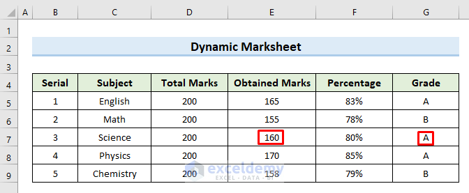
- If we change the marks in cell E7 from 144 to 160, the grade will automatically change from B to A.
The conditions that we have used in the formula:
If the percentage is > 80%, it will return A, if the percentage is < 80%, it will return B, if the percentage is < 60%, it will return C, and if the percentage is < 40%, it will return F.
Read More: How to Calculate Grade Percentage in Excel
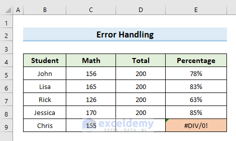
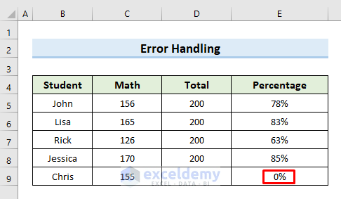
Method 7 – Error Handling While Using Percentage Formulas in Excel
In the following dataset, we face an error in the last row because cell value D9 is missing.
Steps:
- Select E5.
- Insert the following formula in that cell:
=IFERROR(C5/D5,0)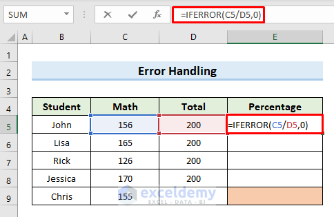
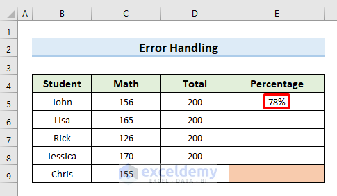
- Press Enter.
- Drag the Fill Handle tool to cell E9.
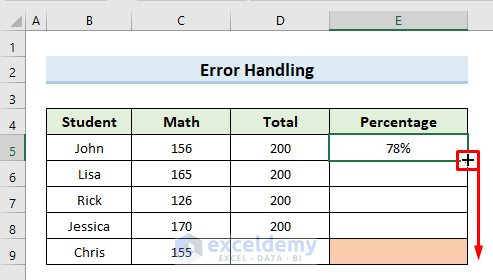
- We can see the value 0 in place of the “#DIV/0”.
Download the Practice Workbook
Related Articles
- Calculate Percentage Using Absolute Cell Reference in Excel
- Calculate Percentage in Excel VBA
- How to Calculate Percentage of Filled Cells in Excel
- IF Percentage Formula in Excel
- How to Calculate Contribution Percentage with Formula in Excel
- How to Calculate Percentage for Multiple Rows in Excel
- How to Use Food Cost Percentage Formula in Excel
- How to Calculate Percentage above Average in Excel
- How to Calculate Variance Percentage in Excel
<< Go Back to Percentage Formula Examples | Calculating Percentages | Calculate in Excel | Learn Excel
Get FREE Advanced Excel Exercises with Solutions!
