Method 1 – Solving Polynomial Equations in Excel
In this section, we will try to solve different polynomial equations like Cubic , Quadratic , linear, etc.
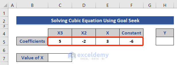
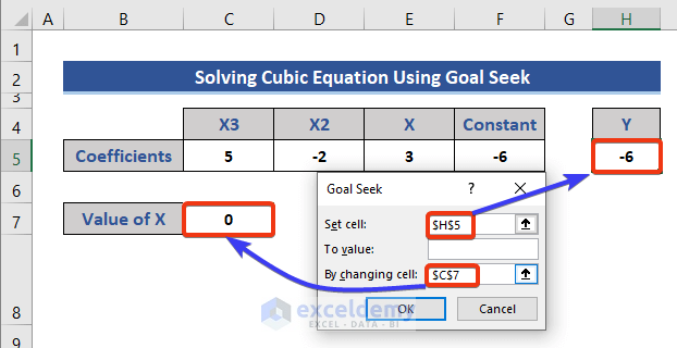
Solving Cubic Equation
Using Goal Seek
We have to solve this equation and find the value of X.
Steps:
- Separate the coefficients into four cells.
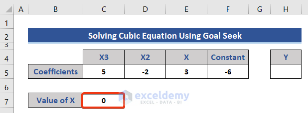
- Assume the initial value of X is zero and insert zero (0) in the corresponding cell.
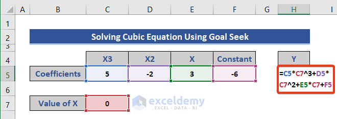
- Formulate the given equation for the cell corresponding to Y.
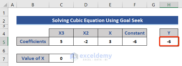
- Press Enter to get the Y value.
=C5*C7^3+D5*C7^2+E5*C7+F5
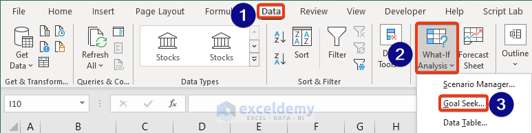
- Click on the Data tab.
- Choose the Goal Seek option from the What-If-Analysis section.
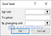
- The Goal Seek dialog box will appear.
- Choose Cell H5 as the Set cell. This cell contains the equation.
- Select Cell C7 as the By changing cell, which is the variable. The value of this variable will change after the operation.
- Put 20 in the To value box, which is a value assumed for the equation.
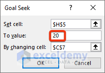
- Press OK.
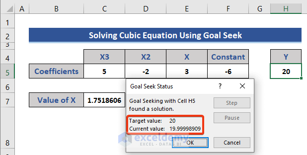
Depending on our given target value, this operation calculates the value of the variable in Cell C7.
- Press OK.
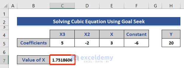
The final value of X is returned.
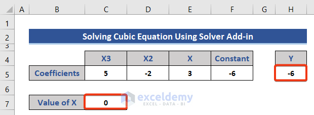
Using Solver Add-In
Steps:
- Set the value of X as zero (0) in the dataset.
- Go to File >> Options.
- Choose Add-ins from the left-hand menu.
- Select Excel Add-ins and click on the Go button.
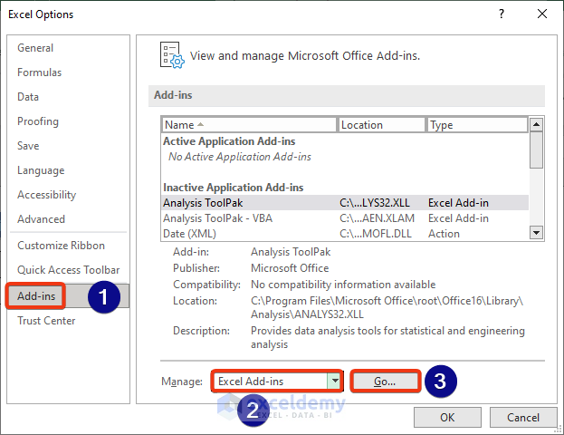
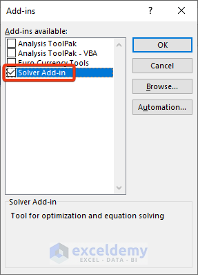
- The Add-ins window appears.
- Check the Solver Add-in option and click OK.
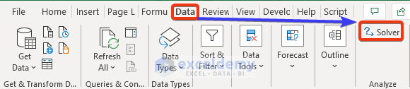
- The Solver add-in has been added to the Data tab.
- Click on the Solver.
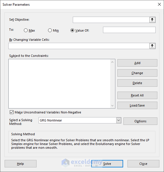
- The Solver Parameters window appears.
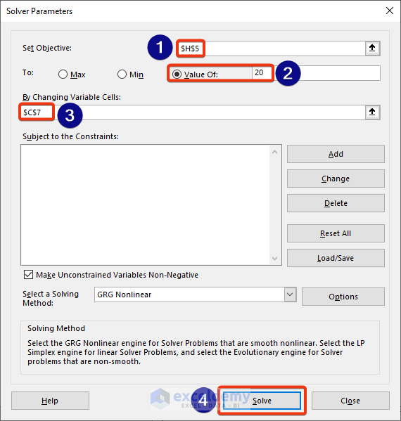
- Insert the cell reference of the equation in the Set Object box.
- Check the Value of the option and put 20 on the corresponding box.
- Insert the cell reference in the variable box.
- Click on Solver.
- Choose Keep Solver Solution and then press OK.

- The value of X has been updated.

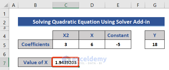
Solving a Quadratic Equation
The following quadratic equation is to be solved.
Solve Using Goal Seek Feature
Steps:
- Separate the coefficients of the variables.
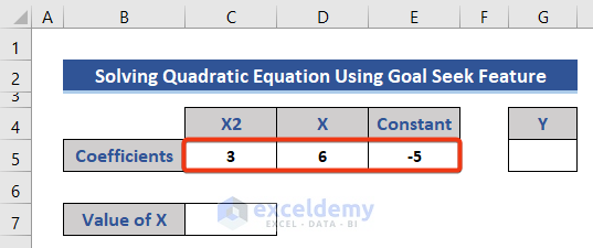
- Set the initial value of X zero (0).
- Insert the given equation using the cell references in Cell G5.
=C5*C7^2+D5*C7+E5
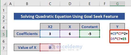
- Press Enter.
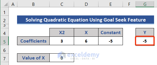
We get a value for Y, assuming X is zero.
- Put the cell reference of the variable and equation in the Goal Seek dialog box.
- Assume the value of equation 18 and put it in the box of the To value section.
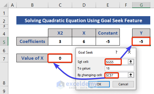
- Press OK.
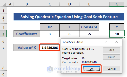
The final value of variable X is returned.
Using Solver Add-In
Steps:
- Enter 0 in Cell C7 as the initial value of X.
- Enter the following formula in Cell G5.
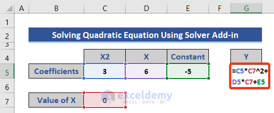
- Press Enter.
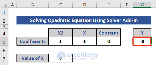
- Select the Solver add-in as shown before.
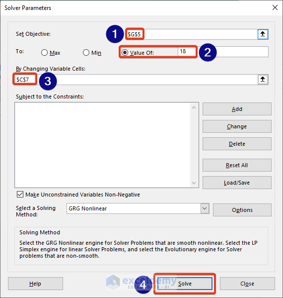
- Choose the cell reference of the equation as the object.
- Enter the cell reference as the variable.
- Set the value of the equation as 18.
- Click on the Solve option.
- Check the Keep Solver Solution option from the Solver Results window.
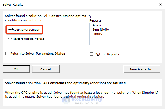
- Click the OK button.
Method 2 – Solving Linear Equations
Using the Matrix System
The MINVERSE function returns the inverse matrix for the matrix stored in an array.
The MMULT function returns the matrix product of two arrays, an array with the same number of rows as array1 and columns as array2.
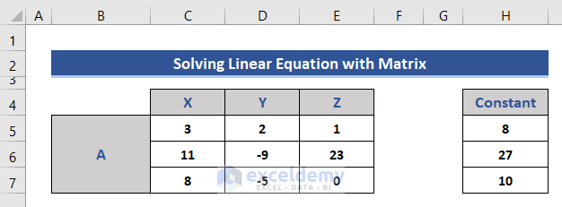
This method will use a matrix system to solve linear equations.
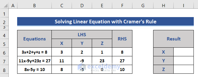
Here, 3 linear equations are given with 3 variables x, y, and z. The equations are:
3x+2+y+z=8,
11x-9y+23z=27,
8x-5y=10
We will use the MINVERSE and MMULT functions to solve the given equations.
Steps:
- Separate the coefficients in the different cells and format them as a matrix.
- Two matrices are created, one with the coefficients of the variable and another one of the constants.
- Add another two matrices for our calculation.
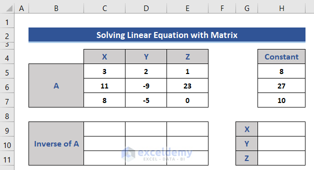
- Find the inverse matrix of A using the MINVERSE function.
- Insert the following formula in Cell C7.
=MINVERSE(C5:E7)
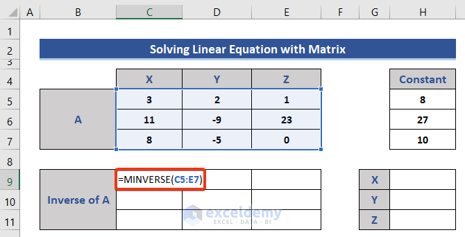
- Press the Enter button.

The inverse matrix is returned.
- Enter the MMULT function in Cell H9.
=MMULT(C9:E11,H5:H7)
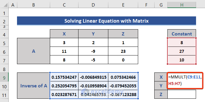
We used a 3x3 and 3x1 matrix in the formula and the resultant matrix is 3x1.
- Press Enter.
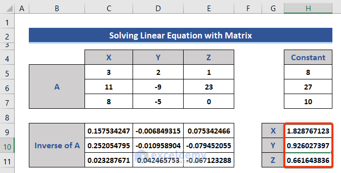
This is the solution of the variables used in the linear equations.
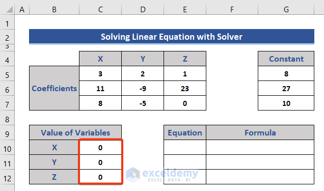
Using Solver Add-In
Steps:
- Separate the coefficients as shown previously.
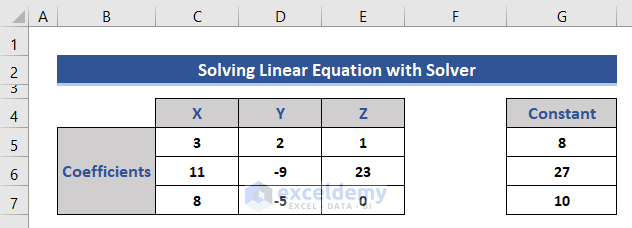
- Add two sections for the values of the variables and insert the equations.
- Set the initial value of the variables to zero (0).
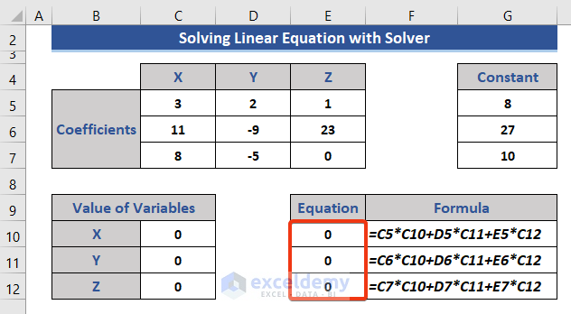
- Insert the following three equations in cells E10 to E12.
=C5*C10+D5*C11+E5*C12
=C6*C10+D6*C11+E6*C12
=C7*C10+D7*C11+E7*C12
- Go to the Solver feature.
- Set the cell reference of the first equation as the objective.
- Set the value of the equation as 8.
- Insert the range of variables in the marked box.
- Click the Add button.

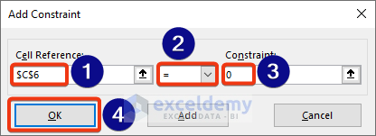
- The Add Constraint window appears.
- Enter the cell reference and values as in the below image.
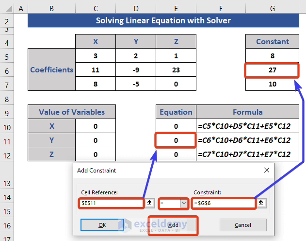
- Insert the second constraint.
- Press OK.
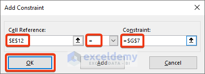
- Constraints are added.
- Press Solve.
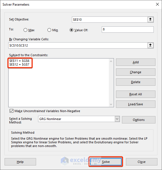
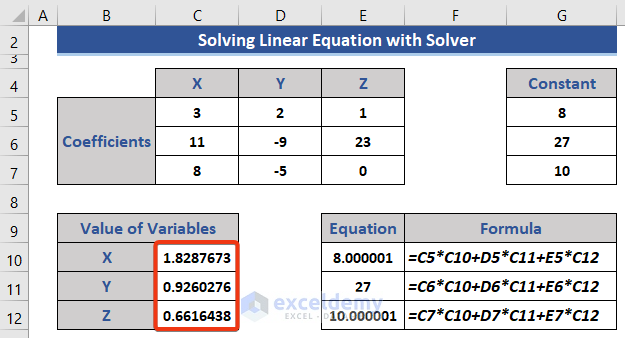
We can see the value of the variables has been changed.
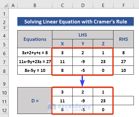
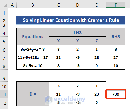
Using Cramer’s Rule for Solving Simultaneous Equations with 3 Variables in Excel
When two or more linear equations have the same variables and can be solved at the same time they are called simultaneous equations. We can solve Simultaneous Equations using Cramer’s rule.
The function MDETERM will be used to find the determinants.
Steps:
- Separate the coefficients into LHS and RHS.
- Add 4 sections to construct a matrix using the existing data.
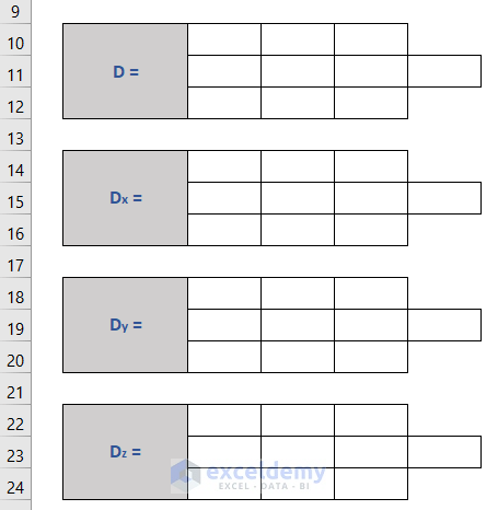
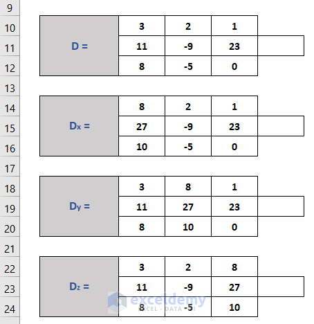
- Use the LHS data to construct Matrix D.
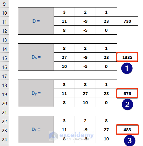
- Construct Matrix Dx by replacing the coefficients of X with the RHS.
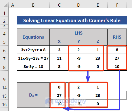
- Repeat to form theDy and Dz matrices.
- Enter the below formula in Cell F11 to get the determinant of Matrix D.
=MDETERM(C10:E12)
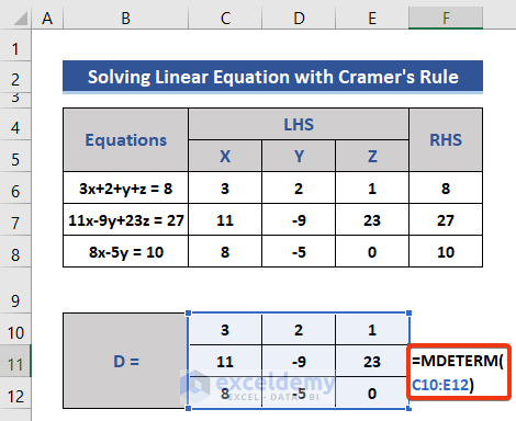
- Press Enter.
- Find the determinants of Dx, Dy, and Dz by applying the following formulas.
=MDETERM(C14:E16)
=MDETERM(C18:E20)
=MDETERM(C22:E24)
- Move to Cell I6.
- Divide the determinant of Dx by D to calculate the value of X.
=F15/F11
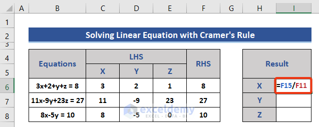
- Press Enter to get the result.
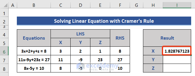
- In the same way, the value of Y and Z are returned using the following formulas:
=F19/F11
=F23/F11
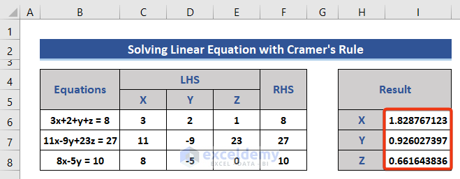
The simultaneous equations have been solved.
Method 3 – Solving Nonlinear Equations in Excel
Steps:
- Insert the equation and variables into the dataset.
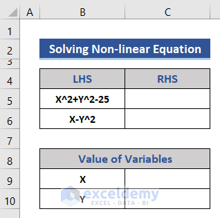
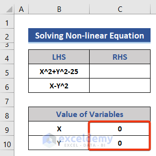
- Set the value of X and Y as zero (0) and insert that into the dataset.
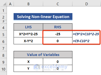
- Insert two equations in Cell C5 and C6 to get the value of the RHS.
=C9^2+C10^2-25
=C9-C10^2
- Add a new row in the dataset for the sum.
- Enter the following equation in Cell C12.
=SUM(C5:C6)
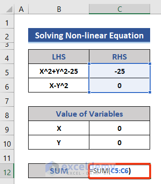
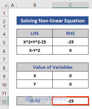
- Press the Enter button to return the sum of the RHS for both equations.
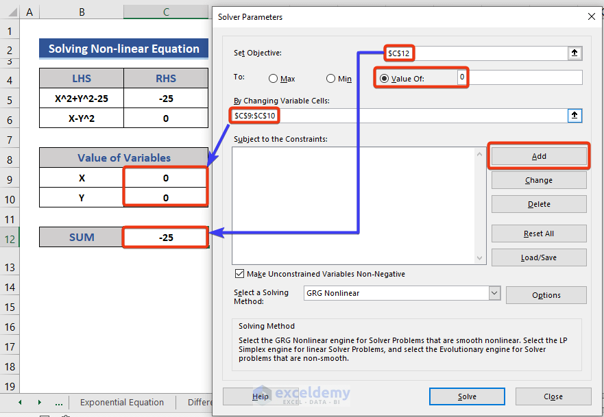
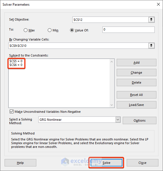
- Apply the Solver feature.
- Insert the cell references in the marked boxes.
- Set the Value of as 0.
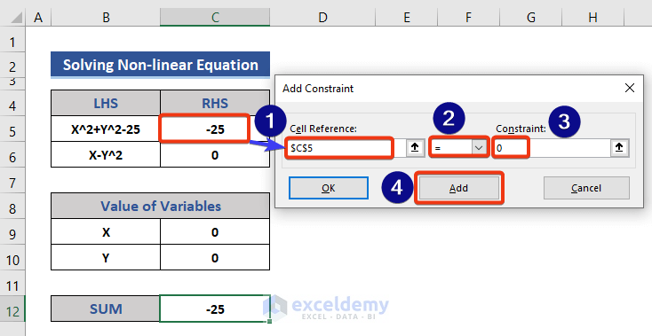
- Click on the Add button to add constraints.
- We add the first RHS as a constraint as shown in the image.
- Press the Add button and add the second RHS.
- Input the cell references and values.
- Press OK.
- We can see constraints are added in the Solver.
- Click the Solver button.
- Check the Keep Solver Solution option and click on OK.
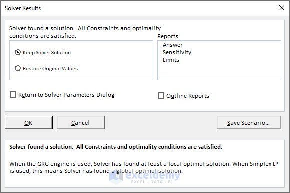
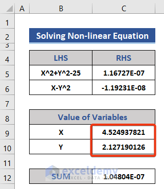
The X and Y values are returned.
Method 4 – Solving an Exponential Equation using the EXP function
We will calculate the future population of an area with a target growth rate using the below equation.
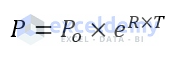
Po= Current or initial population
R= Growth rate
T= Time
P= Esteemed for the future population.
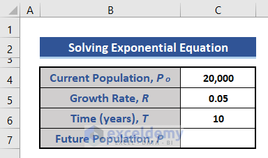
Steps:
- The sample dataset contains current population, target growth rate, and years. The future population is calculated using those values.
- Enter the following formula in Cell C7.
=ROUND(C4*EXP(C5*C6),0)
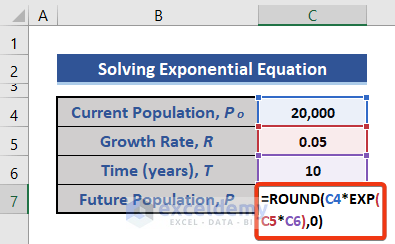
The ROUND function is used as the population must be an integer.
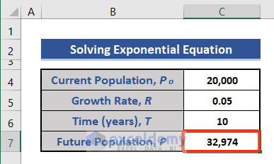
- Press Enter.
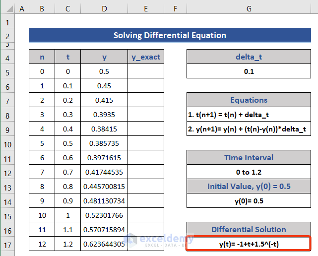
Method 5 – Solving Differential Equations in Excel
In this example we have to find dy/dt, differentiation of y concerning t.
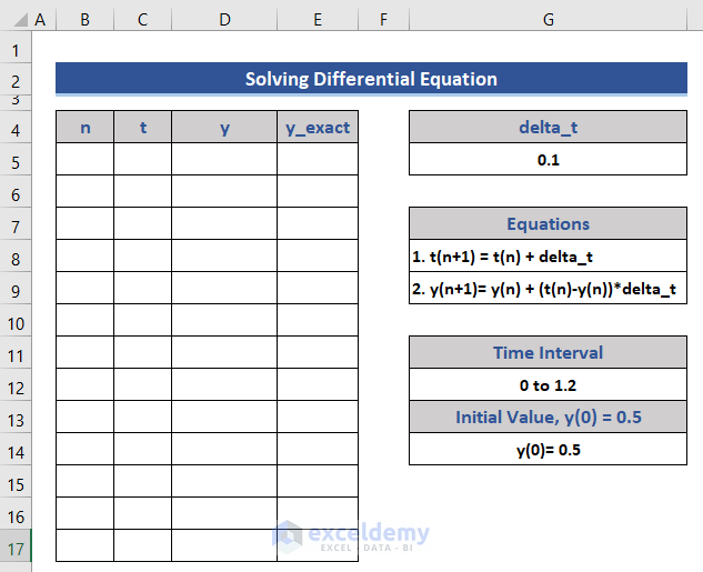
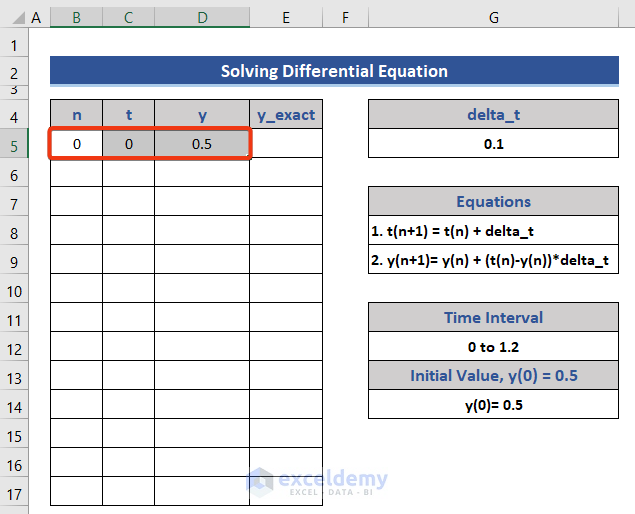
Steps:
- Enter the value of n, t, and y from the given information.
- Enter the following formula in Cell C6 for t.
=C5+$G$5
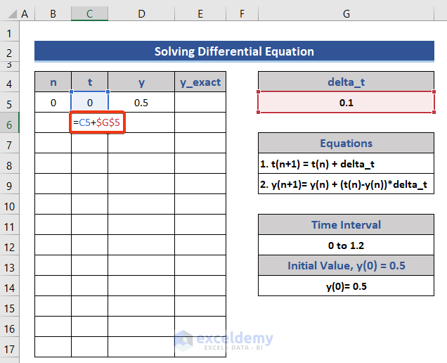
This formula has been generated from t(n-1).
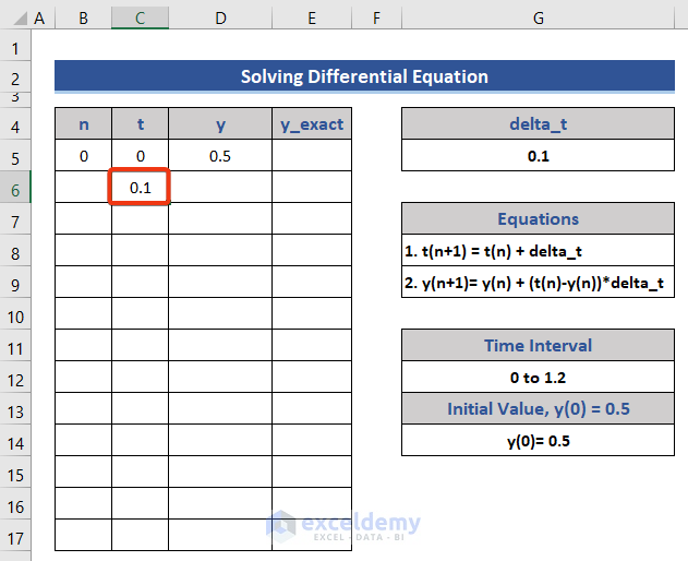
- Press the Enter button.
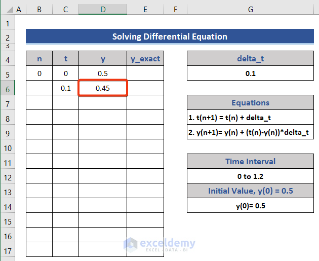
- Enter the below formula in Cell D6 for y.
=D5+(C5-D5)*$G$5
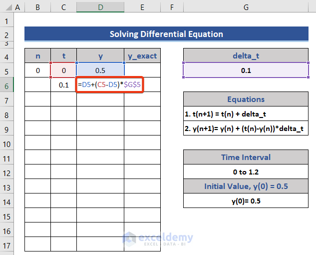
- Press Enter.
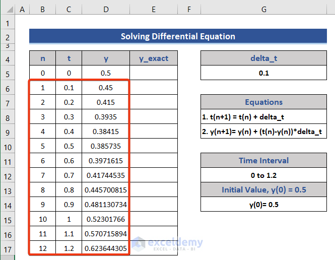
- Extend the values to the maximum value of t, which is 1.2.
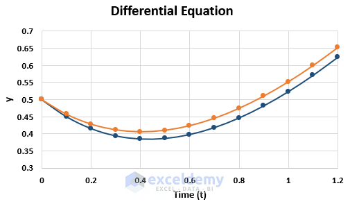
Draw a graph using the values of t and y.
- Go to the Insert tab.
- Choose a graph from the Chart group.
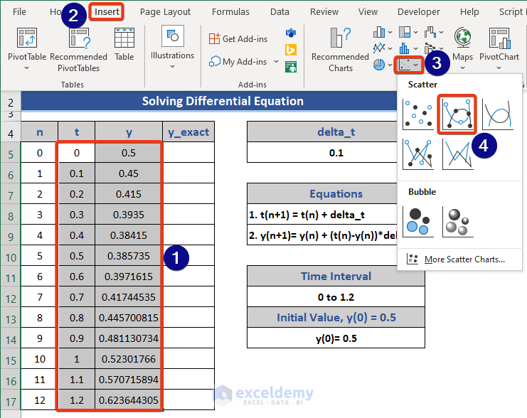
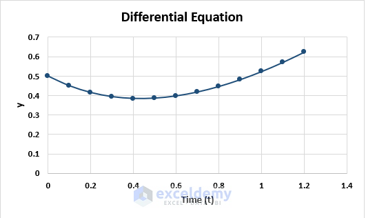
The graph plots y versus t.
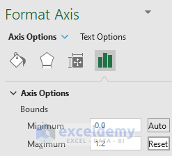
- Double-click on the graph and select the minimum and maximum values of the graph axis. Reset the horizontal line.
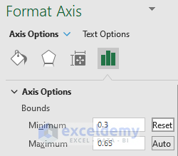
- Reset the vertical line.
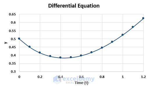
- After customizing the axis, our graph looks like this.
- Calculate the differential equation manually and put it on the dataset.
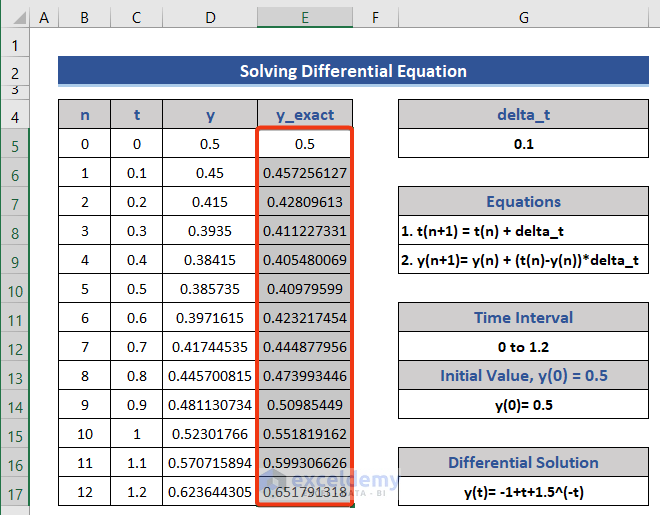
- Enter the below formula in Cell E5.
=-1+C5+1.5*EXP(-C5)
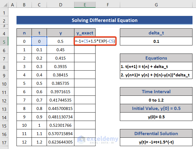
- Press the Enter button and drag the Fill Handle icon.
- Right click on the graph.
- Choose the Select Data option from the Context menu.
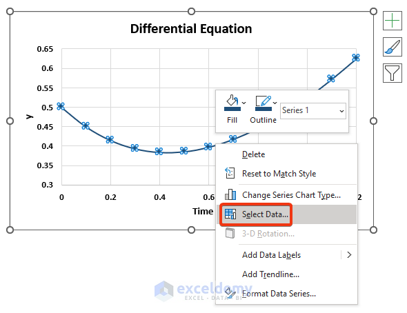
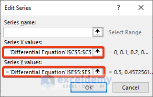
- Select the Add option from the Select Data Source window.
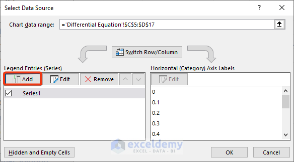
- Choose the cells of the t column as X values and cells of the y_exact column as Y values in the Edit Series window.
Download Practice Workbook
Excel Solver Examples: Knowledge Hub
- How to Solve for x in Excel
- How to Solve an Equation for X When Y is Given in Excel
- How to Solve 2 Equations with 2 Unknowns in Excel
- How to Solve Algebraic Equations with Multiple Variables
- How to Solve System of Equations in Excel
- How to Solve Colebrook Equation in Excel
<< Go Back to Excel Solver Examples | Solver in Excel | Learn Excel
Get FREE Advanced Excel Exercises with Solutions!

why have stooped “Download Article in PDF Format option”
Thanks for asking. It was creating more indexed pages in Google that was bad for us. What you can do is: just you can copy the whole article and paste into a word document and then convert it into a PDF file. There is little chance of getting back of that button.
Best regards
I have a few points that when graphed LOOK like a quadratic equation. How do I go from the set of points to get EXCEL to deliver an EQUATION for the quadratic function given those points (like it can do for LINEAR equations)?
Hello SHAWN S FAHRER!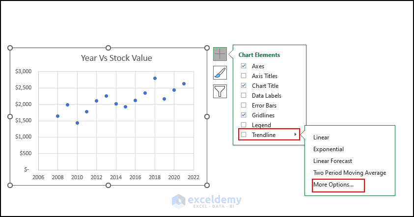
You can get a quadratic equation from a graph with a few points that you have mentioned here. Follow the steps below for this
First, create a graph with the points you have.
Then, Go to the Chart Elements clicking the Plus icon.
Click on the arrow beside the “Trendline” option.
Go to the “More Options”
1
Here, you will go to a window named “Format Trendline”.
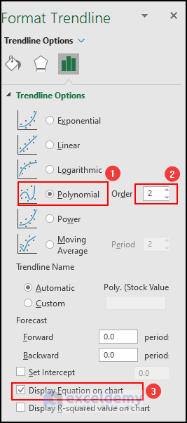
Select the “Polynomial” option of order 2.
Mark the checkbox saying “Display Equation on Chart”.
As a result, you will there will create a trend line following a quadratic equation which is also shown in the graph.
Try this method and let us know the outcome! Thank You!
Hi thanks for posting this article. Can you please elaborate on why did you assume 15 as the value of Y? By definition, shouldn’t we be solving for 3 values of x as the equation is cubic?
Hello MANUJ! You have to insert a value as the set value for cell G3 to use Goal Seek feature.. suppose you have an equation like 5x^3 – 2x^2 + 3x – 21 = 0 then you can change the equation like 5x^3 – 2x^2 + 3x – 6 = 15. Here, we have done this.
And, yes! you are right that the cubic function gives 3 root values. But using the Goal Seek Feature, you will get only one root. and, in many times, the cubic function may have one real root and 2 complex roots. In these cases, the goal seek feature will give the value of the real root.
Try these examples and let us know the output. Thank You!