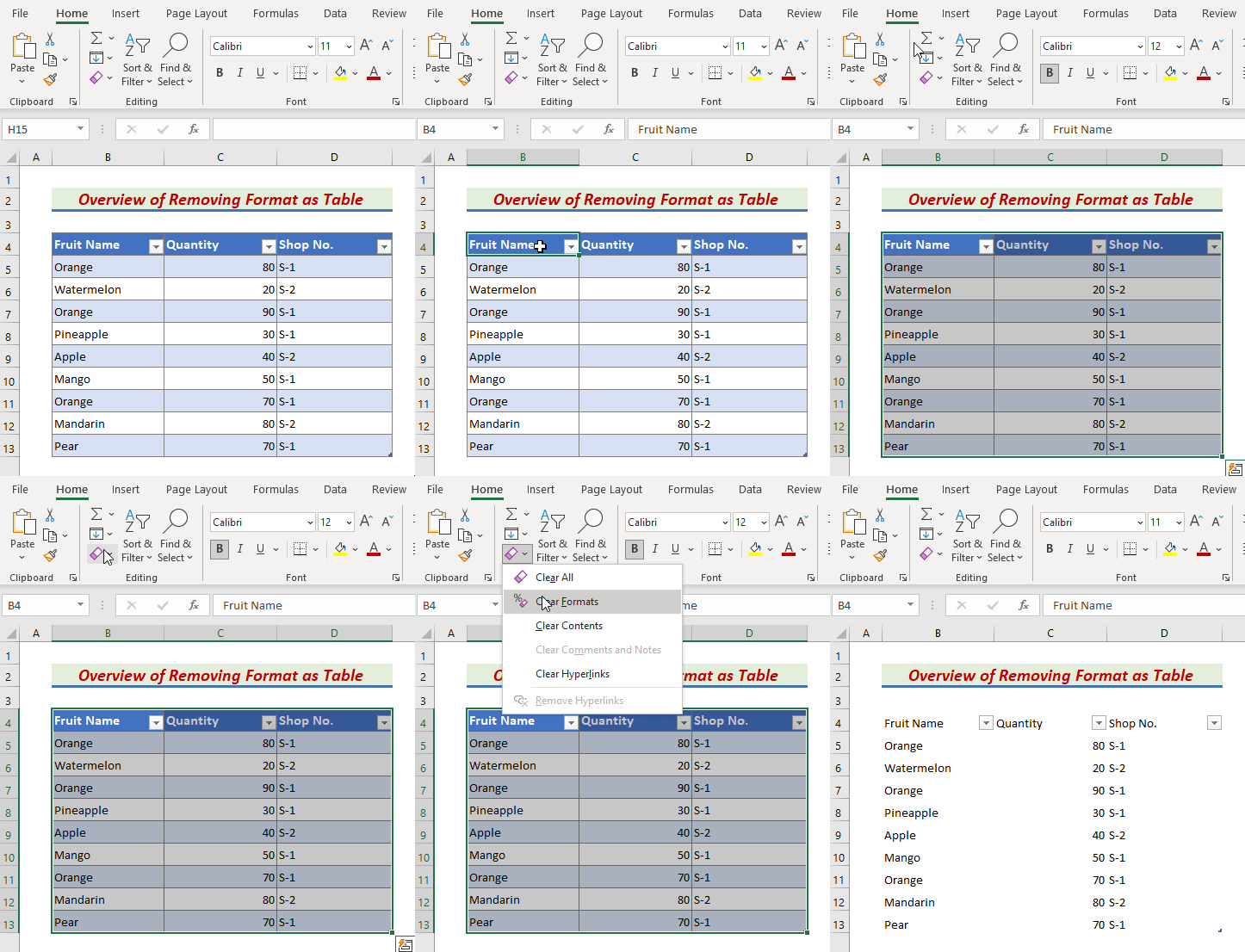
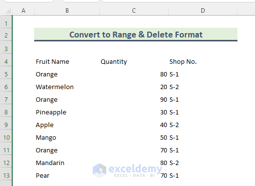
While working in Excel, we often apply different types of styles and formatting in table cells. Most of the time, these formats are helpful. But, at times, they can be distracting too. Fortunately, there are some very easy and quick ways to erase the format as a table in our Excel dataset. With this in mind, we will discuss 3 suitable methods to remove the format as the table in Excel. Take a look at the overview of this article below for a better understanding.
Remove Format As Table in Excel: 3 Quick Methods
1. Delete Format from Table Design Tab in Excel
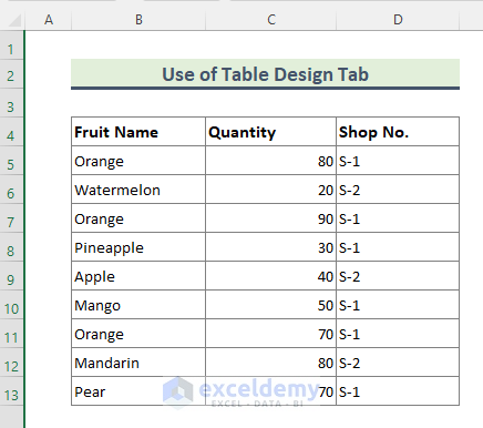
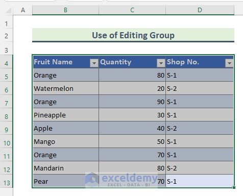
Before removing formatting from a table, let’s create a table from a date range. Suppose we have a data range containing fruit sales details.
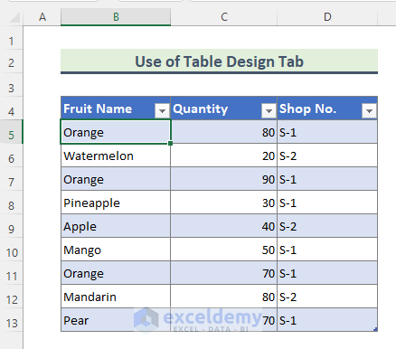
To create a table from this data range just select the data and type Ctrl+T. The table will be created with default formatting.
Now, we will go through the steps to delete this formatting.
Steps:
- First, select any cell of the table.
- Next, go to Table Design. This is a Contextual tab that only appears when a table cell is selected.
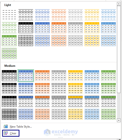
- Then, go to the Table Styles group and click on the More icon (down to the right side scroll bar).
- After that, click on the Clear option.
- Finally, the table is free of all types of auto-generated formats.
If you apply any formatting manually to the table, those won’t be removed using the above method.
Read More: How to Remove Table in Excel
2. Remove Format as Table from Editing Group in Excel
Now, we will explain another method regarding removing format from an Excel table.
Steps:
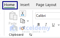
- Next, go to the Home tab from the Ribbon.
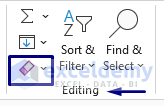
- Then, go to the Editing group and click on the Clear
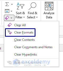
- After that, click on the Clear Formats option from the Clear drop-down.
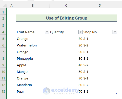
- Lastly, all the formats from the table will be deleted.
Read More: How to Remove Table Functionality in Excel
3. Convert Table to Range and Clear Format in Excel
Sometimes we need to convert tables to data range and then clear the formats. Now, we will discuss the steps involved in that process.
Steps:
- First, select any cell of the table.
- Next, go to the Table Design Tab and click on Convert to Range from the Tools group.
- After that, the Microsoft Excel window will pop up to confirm the table-to-range conversion. Click Yes.
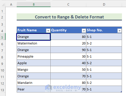
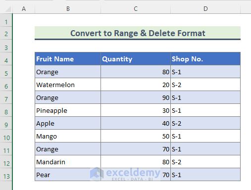
- Then, the table will be converted to a data range. Yet, all the formatting is present.
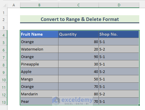
- Now, select the entire data range and follow the steps mentioned in Method 2.
(Go to Home > Clear (Editing Group) > Clear Formats)
- Finally, here is the data range, free of any formatting.
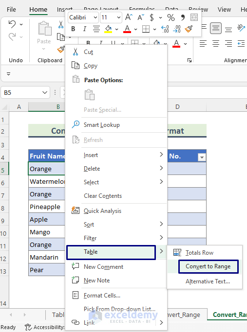
You can convert tables into data ranges through a right-click also. To do this, right-click any cell of the table, and then from the Table option, click on Convert to Range.
Read more: Excel Table Formatting Problems
Download the Practice Workbook
You can download the practice workbook that we have used to prepare this article.
Conclusion
In the above article, we elaborately discussed all the methods to remove format as the table in Excel. Hopefully, these methods and explanations will be enough to solve your problems. Please let me know if you have any queries.
Further Readings
- How to Make an Excel Table Expand Automatically
- How to Use Sort and Filter with Excel Table
- How to Insert or Delete Rows and Columns from Excel Table
- How to Mirror Table in Excel
- [Fix]: Formulas Not Copying Down in Excel Table
- How to Rename a Table in Excel
- How to Extend Table in Excel
- How to Undo a Table in Excel
<< Go Back to Change Table Style | Make an Excel Table | Excel Table | Learn Excel
Get FREE Advanced Excel Exercises with Solutions!