Gridlines are a classical feature of spreadsheets. In Excel, gridlines help the user to distinguish between cells and navigate within the rows and columns. However, the gridlines disappear as soon as we apply the Fill Color feature to color the cells. In this article, we’ll show you 4 simple ways to print gridlines in Excel with fill color.
How to Print Gridlines with Fill Color in Excel: 4 Ways
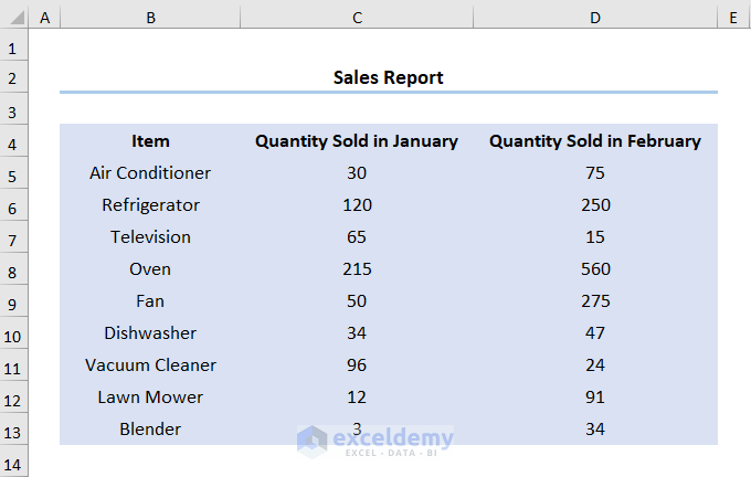
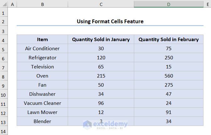
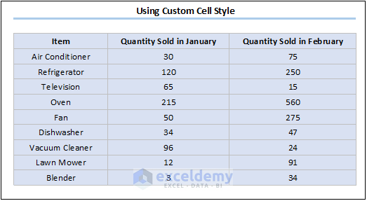
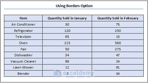
Firstly let’s consider the Sales Report dataset in the B4:D13 cells. Here, the report shows the sales of various Items and their Quantities Sold for the month of January and February. Now, we want to show the Gridlines and the Fill Color when we print this dataset. So, without further delay, let’s see the methods one by one.
We have used Microsoft Excel 365 version here, you can use any other versions according to your convenience.
Method-1: Employing Format Cells Feature to Print Gridlines with Fill Color
Let’s begin with the most obvious way of adding Gridlines and Fill Colors in Excel. Yes, you’ve guessed it correctly. We’ll use the Format Cells feature. Therefore, just follow these steps.
Steps:
- Initially, select the range of cells B4:D13 >> now, press CTRL + 1 on your keyboard.
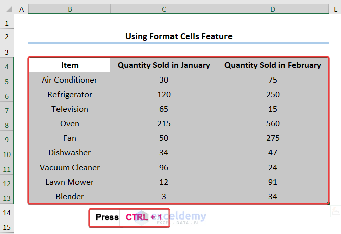
This opens the Format Cells dialog box.
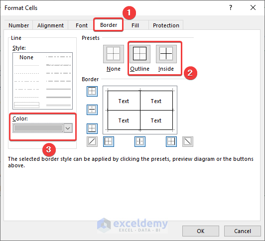
- Next, go to the Border tab >> click the Outline and Inside buttons respectively >> select a Color (here, we chose Grey).
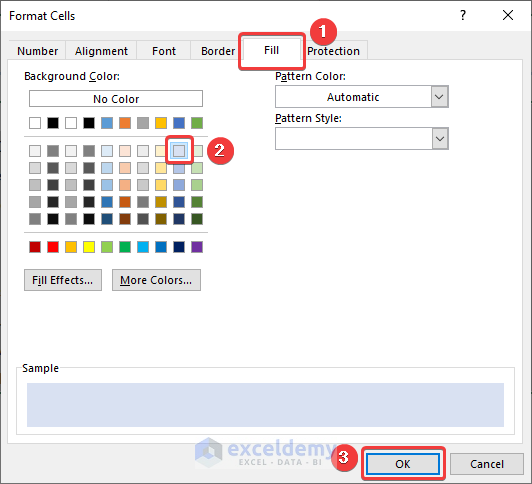
- Following this, move to the Fill tab >> select a Fill Color for the cells, for instance, we chose a Light Blue color >> lastly, press the OK button.
This should return the results shown in the picture below.
- Moreover, press CTRL + P to check the Print preview before printing.
That’s it you’ve added the Fill Color and preserved the Gridlines. It’s that easy!
Read More: How to Print Gridlines in Excel Online
Method-2: Utilizing Custom Cell Style
Excel allows you to create a custom Cell Style where you can show the Gridlines and add Fill Color to your worksheet. Now, allow me to demonstrate the process in the steps below.
Steps:
- To start, navigate to the Home tab >> in the Styles section, and click the Arrow button.
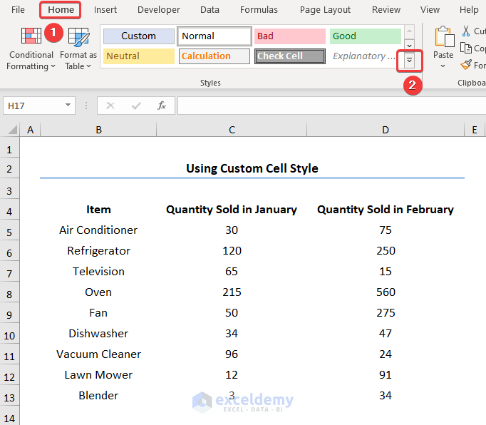
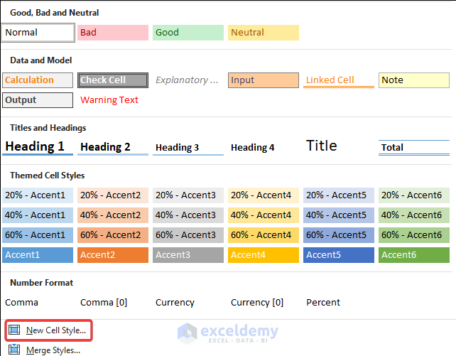
- Now, select the New Cell Style option at the bottom.
This opens the Style wizard.
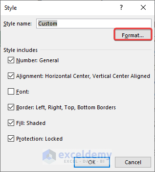
- Next, enter a name in the Style name field, for example, here, it is Custom.
- Then, press the Format button.
After completing the previous step, the Format Cells dialog box pops up.
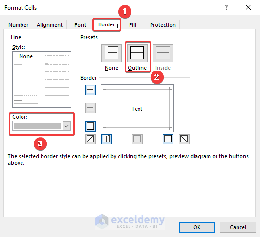
- In turn, move to the Border tab >> click the Outline button>> select a Color (for example, we chose Grey).
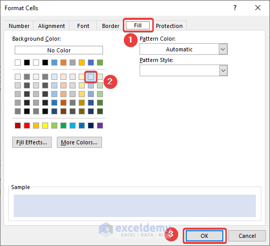
- In the next step, go to the Fill tab >> select a Fill Color for the cells (here, it is Light Blue) >> click the OK button.
- In the last step, select the B4:D13 cells >> click the Custom style in the Styles section.
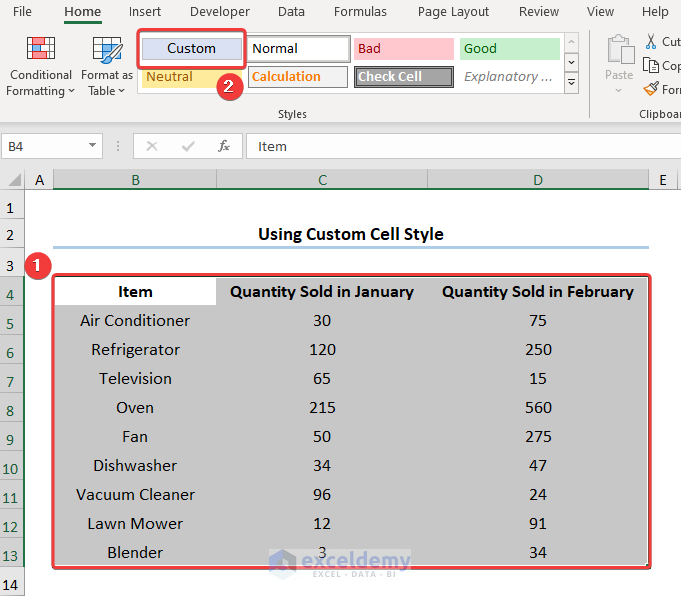
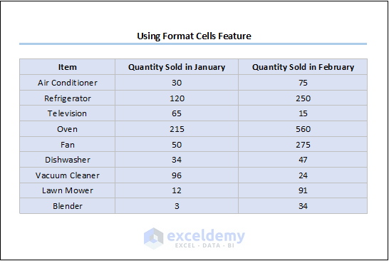
You’ll see the output as shown in the screenshot below.

- In addition, press CTRL + P to preview the results before printing.
Read More: How to Print Excel Sheet with Lines
Method-3: Using Borders Option to Print Gridlines with Fill Color in Excel
If the previous methods are too much work and you’re in a hurry then, out third method may be the answer to your prayers! It’s simple and easy. Hence, let’s see it in action.
Steps:
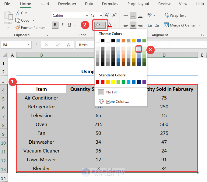
- Firstly, select the range of cells B4:D13 >> now, click the Fill Color drop-down to pick a color of your choice (like we chose Light Blue).
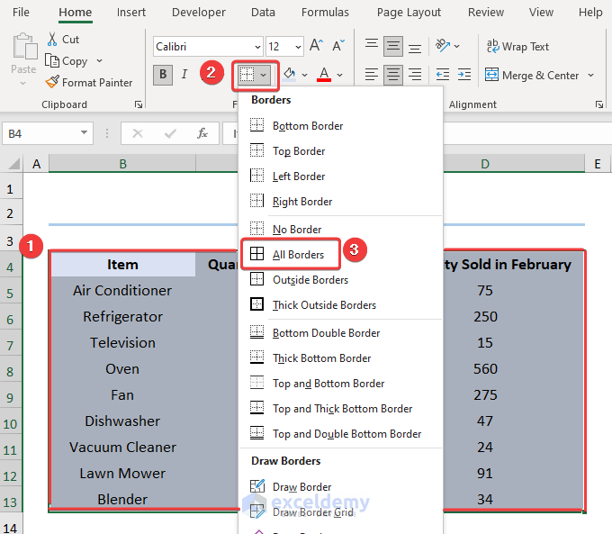
- Secondly, move to the Borders drop-down and choose the All Borders option.
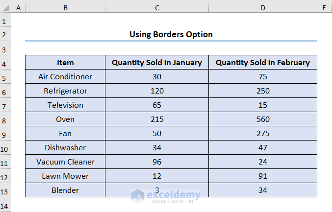
This should generate the results like the image given below.
- Thirdly, press CTRL + P to check the output before printing.
Read More: How to Print Excel with Lines on One Page
Method-4: Applying VBA Code to Print Gridlines with Fill Color
If you often need to get the column number of matches, then you may consider the VBA code below. It’s simple & easy, just follow along.
Step-01: Open Visual Basic Editor
- Firstly, navigate to the Developer tab >> click the Visual Basic button.
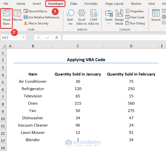
This opens the Visual Basic Editor in a new window.
Step-02: Insert VBA Code
- Secondly, choose ThisWorkbook option >> next, go to the Insert tab >> select Module.
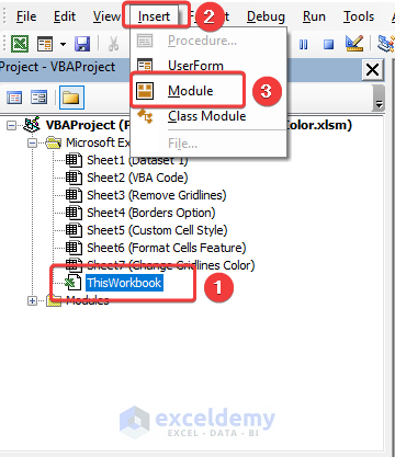
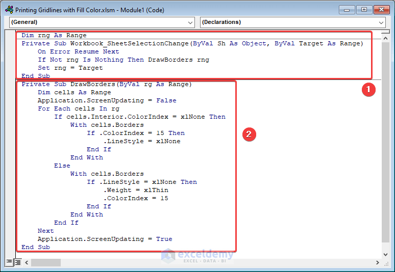
For your ease of reference, you can copy the code from here and paste it into the window as shown below.
Dim rng As Range
Private Sub Workbook_SheetSelectionChange(ByVal Sh As Object, ByVal Target As Range)
    On Error Resume Next
    If Not rng Is Nothing Then DrawBorders rng
    Set rng = Target
End Sub
Private Sub DrawBorders(ByVal rg As Range)
    Dim cells As Range
    Application.ScreenUpdating = False
    For Each cells In rg
        If cells.Interior.ColorIndex = xlNone Then
            With cells.Borders
                If .ColorIndex = 15 Then
                    .LineStyle = xlNone
                End If
            End With
        Else
            With cells.Borders
                If .LineStyle = xlNone Then
                    .Weight = xlThin
                    .ColorIndex = 15
                End If
            End With
        End If
    Next
    Application.ScreenUpdating = True
End Sub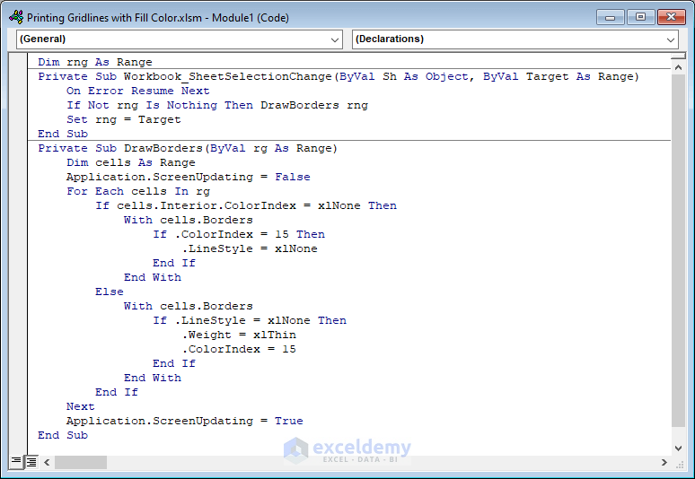
Code Breakdown:
Now, I will explain the VBA code for preserving Gridlines in Fill Color. In this case, the code is divided into two steps.
- Firstly, in the first portion, define the variable rng.
- Next, define the sub-routine Workbook_SheetSelectionChange() and its arguments Sh and Target.
- Then, use an If statement to add borders in the chosen range of cells.
- Secondly, in the latter part, define the sub-routine DrawBorders() and its argument rg.
- Now, iterate within the chosen range of cells using the For statement.
- Following this, nest If statements within the For statement and insert borders using the Borders property.
- Likewise, specify the style and line-width with LineStyle and Weight properties.
- Finally, set the ScreenUpdating property to True.
Step-03: Running VBA Code
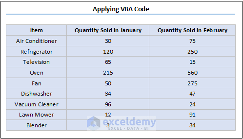
- Finally, close the VBA window >> now, highlight the range of cells in B4:D13 >> choose a Fill Color (here, it is light blue) >> you’ll see the Gridlines remain visible.

- Additionally, press CTRL + P to check the preview before printing.
The result should look like the image shown.
Read More: [Fixed!] Missing Gridlines in Excel When Printing
Removing Gridlines from Worksheet
Excel makes removing gridlines very easy. So, just follow these steps.
Steps:
- Firstly, navigate to the View tab >> by default, the Gridlines option is checked, just uncheck the option.
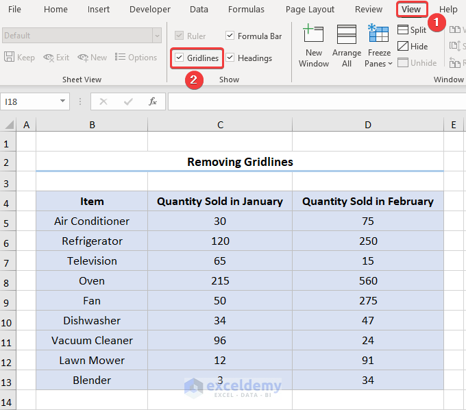
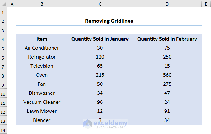
That’s it the Gridlines have vanished. Needless to say, you can check the box to show the Gridlines again.
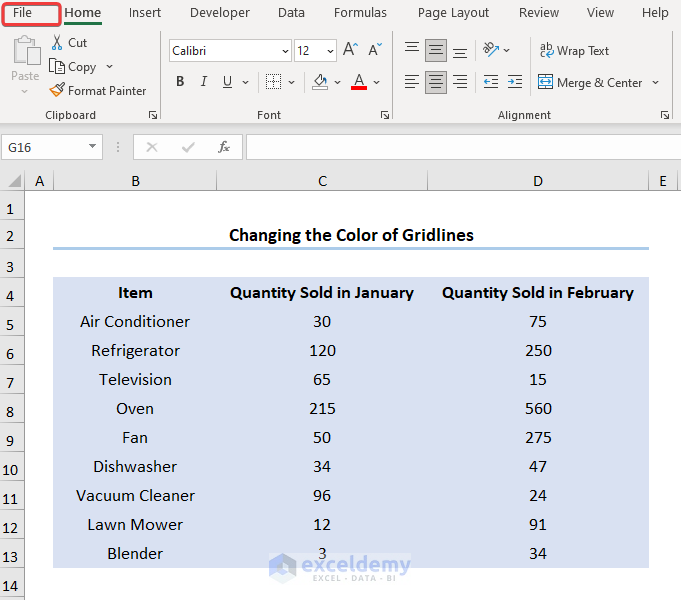
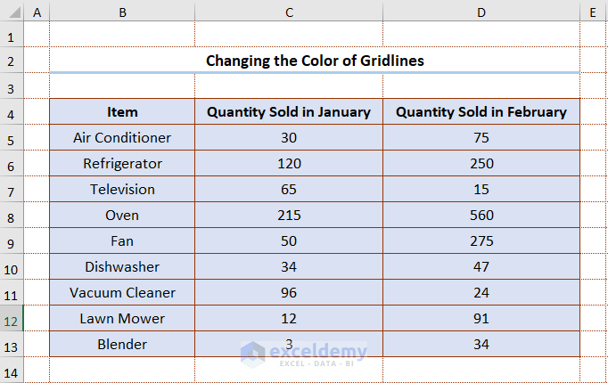
Changing Color of Gridlines in Excel
You can spice up your dataset by changing the monotonous color of the Gridlines. It doesn’t take a lot of time and effort. Therefore, let’s see it in action.
Steps:
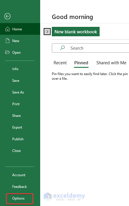
- Firstly, navigate to the File tab.
- Now, click the Options button at the bottom.
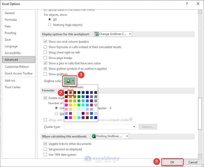
- Secondly, go to the Advanced section >> scroll down to the Display options for this worksheet >> choose the current worksheet (here, it is Change Gridlines Color).
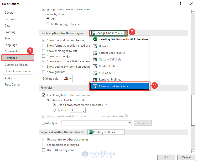
- Thirdly, specify the Gridline color, for instance, we chose Brown.
- Next, click the OK button.
Eventually, the Gridline colors of the current worksheet should look like the picture shown below.
Practice Section
For doing practice by yourself we have provided a Practice section like below in each sheet on the right side. Please do it by yourself.

Download Practice Workbook
You can download the practice workbook from the link below.
Conclusion
This article answers how to print gridlines with fill color in Excel in a quick and easy way. Make sure to download the practice file from above. Hope you found it helpful. Please inform us in the comment section about your experience. Keep learning and keep growing!
Related Articles
<< Go Back to Print Gridlines | Print in Excel | Learn Excel
Get FREE Advanced Excel Exercises with Solutions!
