In this tutorial, I am going to show you 4 quick tricks on how to hide gridlines in Excel when printing a worksheet. Although Excel hides the gridlines when printing as default, you may get some file from other sources where you have the gridlines visible. In this case, you use the following methods to hide those gridlines.
How to Hide Gridlines in Excel When Printing: 4 Quick Tricks
1. Using Sheet Options
MS Excel provides multiple sheet options for printing purposes. We will use one of it’s useful features to hide the gridlines in excel when printing.
Steps:
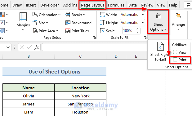
- First, go to the Page Layout tab and then Sheet Options.
- Here, under the Gridlines section, uncheck the option Print.
- Next, go to the File tab.
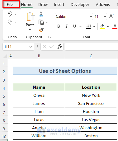
- Then, from the left column options select Print.
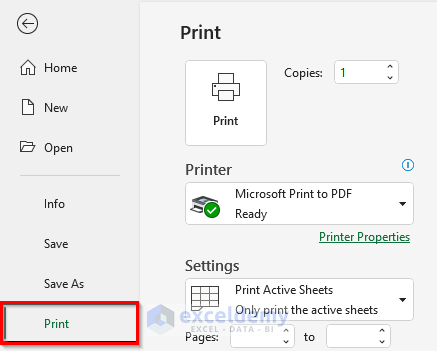
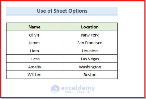
- Finally, you will see that the gridlines are hidden in the print preview.
Read More: How to Print Gridlines in Excel Online
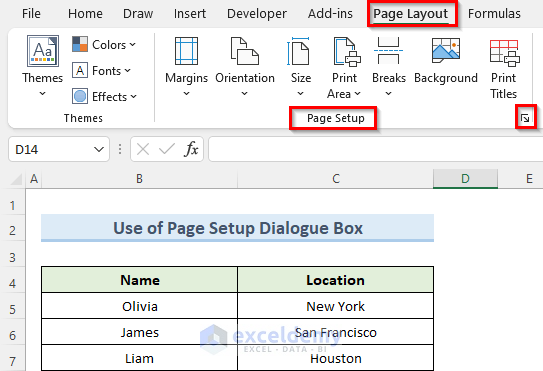
2. Utilizing Page Setup Dialogue Box
We can use the Page Setup dialogue box to customize the elements of our excel worksheet. Let us see how we can hide the gridlines in excel when printing using this feature.
Steps:
- To begin with, go to the Page Layout tab and then Page Setup.
- Now, click on the arrow at the lower-right corner of this section as shown below.
- Next, in the Page Setup window, go to the Sheet tab.
- Now, under the Print section, uncheck the option Gridlines.
- Finally, press OK and excel will hide the gridlines when printing this worksheet.

Read More: How to Print Excel Sheet with Lines
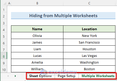
3. Hiding Gridlines from Multiple Sheets When Printing
When you have quite a few excel worksheets and you need to hide the gridlines from all of them, then this method can be helpful.
Steps:
- To start with, go to the bottom of your workbook.
- Here, on the Status Bar, hold Ctrl and select the sheets that you want to hide gridlines in.
- Next, go to the Page Layout tab as we did previously.
- Then, under the Gridlines section, simply uncheck the option Print.
- Finally, this will hide the gridlines from the printed worksheets that you selected.

Read More: How to Print Excel with Lines on One Page
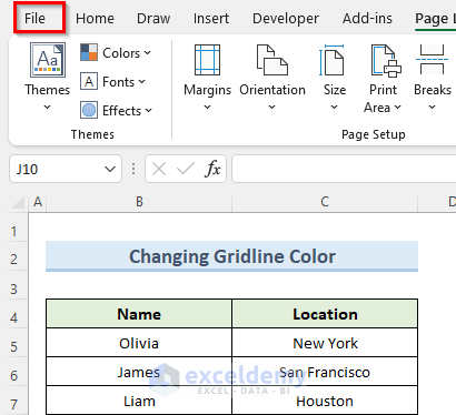
4. Changing Gridlines Color
This method in reality will not hide the gridlines. Rather it will change the default printing color of the gridlines. Let us see how we can apply this method.
Steps:
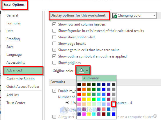
- First, navigate to the File tab at the top-left corner of your screen.
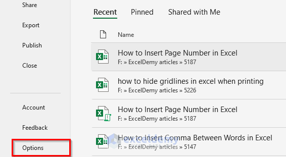
- Next, click on Options.
- Then, in the Excel Options window, go to Advanced.
- Now, navigate to the section Display options for this worksheet and change the Gridline color to White. Press OK.
- As a result, the gridlines will become invisible when printing.
Read More: How to Print Gridlines with Fill Color in Excel
How to Show Gridlines in Excel When Printing
As we said previously, by default excel keeps the gridlines hidden when printing. So if you need to make the gridlines visible, you can follow the steps below.
Steps:
- First of all, go to the Page Layout tab and then to Sheet Options.
- Now, under the Gridlines section, check the Print option, just as the opposite of what we did previously.
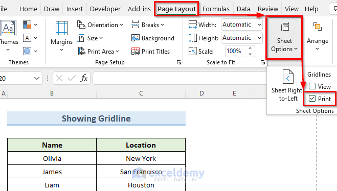
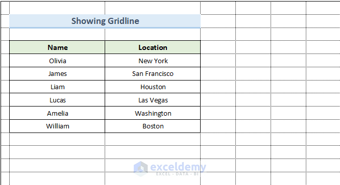
- Finally, go to print preview and you will see the gridlines now showing on the worksheet.
Download Practice Workbook
You can download the practice workbook from here.
Conclusion
I hope that the methods I showed in this brief tutorial on how to hide gridlines in excel when printing was helpful to you. Note that, if you turn off the gridlines when viewing the worksheet, they will still be visible when printing. Also, among the methods that I showed, you should choose the one that best fits your need. Moreover, whether you want to hide or show the gridlines when printing, depends totally on your situation. If you have any queries, please let me know in the comments.
Related Articles
<< Go Back to Print Gridlines | Print in Excel | Learn Excel
Get FREE Advanced Excel Exercises with Solutions!
