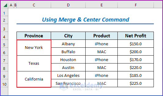
In this article, we will demonstrate the methods available in Excel to merge two consecutive rows into one single row. We’ll use the dataset below, containing 4 columns with the net profit of some products in different areas, to illustrate the methods.
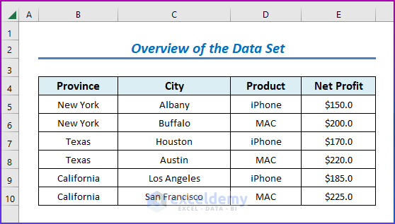
We’ll merge rows to produce two different outputs: Losing Data & Keeping Data Intact.
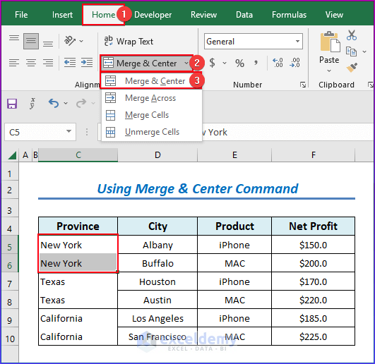
Method 1 – Using Merge & Center Command (Loses Data)
Here, we will merge the names of the Provinces into one row using the Merge & Center feature.
Steps:
- Go to the Home tab
- From the Alignment group, click Merge & Center.
- Click on the Merge & Center command.
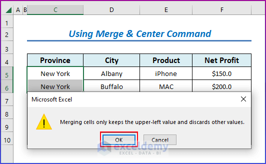
A warning window will pop up.
- If you explicitly know that losing the data will not hamper you, then click OK.
The merged text New York is returned.
- Apply the Merge & Center command for the rest of the cells.
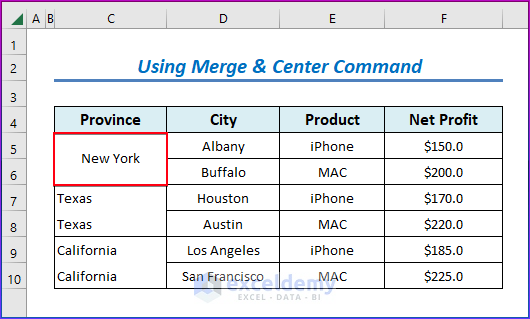
The output is as in the below image.
Read More: How to Combine Multiple Rows into One Cell in Excel
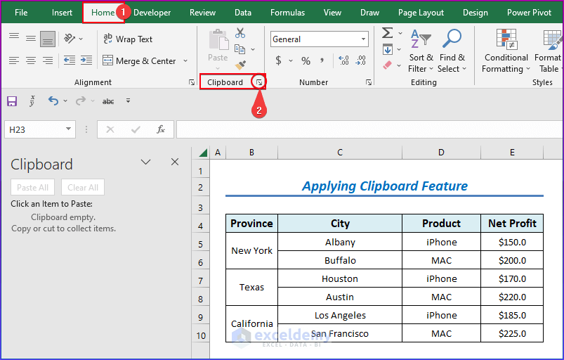
Method 2 – Using Excel Clipboard Feature (Keeps Data Intact)
Steps:
- In the Home tab, in the Clipboard section, click the Arrow Icon.
The Clipboard Window will appear on the left side of the workbook.
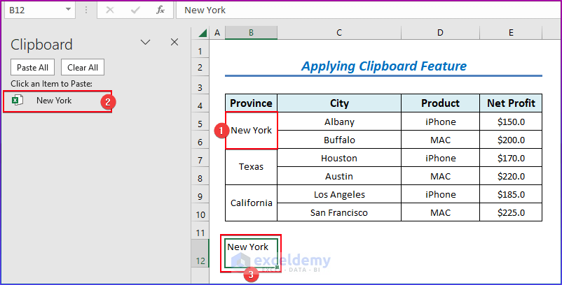
- Select the two Rows and press Ctrl+C (copy).
- Select any cell, double-click on it, and Click on the available Item to Paste.
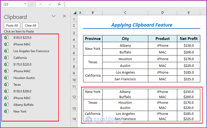
After further application of the command sequence for the rest of the rows, the outcome will be as in the below image.
Method 3 – Applying CONCATENATE Function (Keeps Data Intact)
The CONCATENATE function or Concatenation Operator is used to merge two or more rows using various delimiter types, which separate the different text values.
Steps:
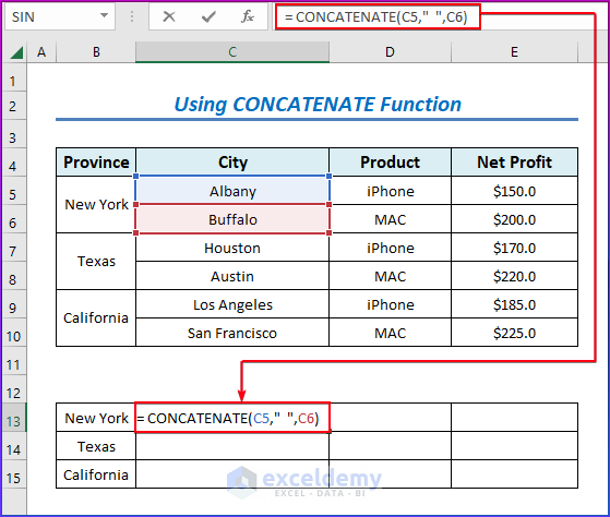
- In cell C13, enter the following formula:
= CONCATENATE(C5," ",C6)Spaces & commas will appear between row texts as shown as in the image below.
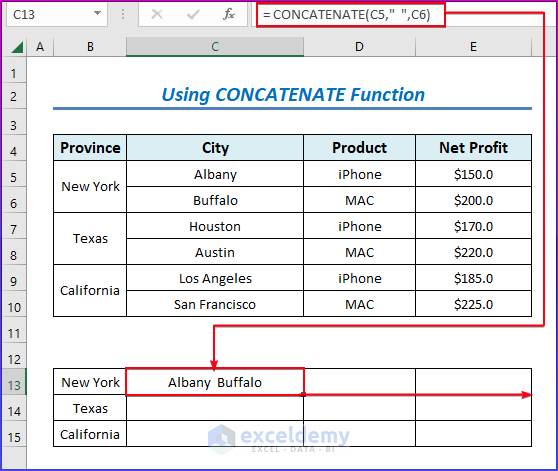
If you want to place a Space between the texts then use [“ ”] as your delimiter.
- Press Enter to return the result in cell C13.
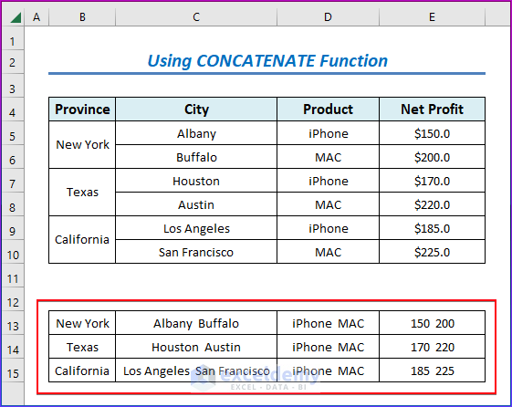
- Use the Fill Handle tool and drag it down from cell C13 to cell C15.
- Apply the same procedure for the 14th and 15th rows.
- The results are as follows:
Read More: How to Merge Rows with Comma in Excel
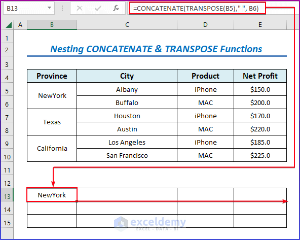
Method 4 – Nesting CONCATENATE & TRANSPOSE Functions (Keeps Data Intact)
A combination of the CONCATENATE & TRANSPOSE functions can also be used to merge two rows of values without losing any data.
Steps:
- In cell C13 cell, enter the following formula:
=CONCATENATE(TRANSPOSE(B5)," ", B6)- Press Enter.
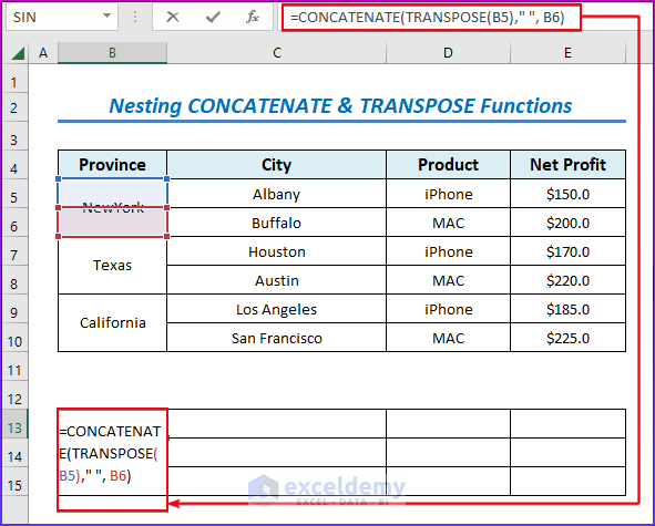
The result is returned in cell C13.
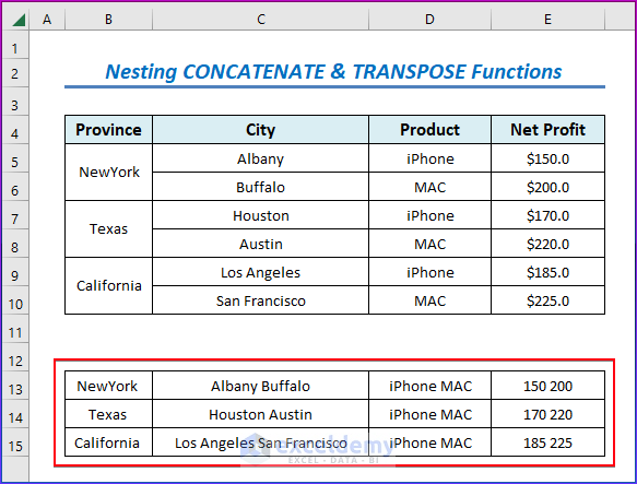
- Use the Fill Handle tool and drag it down from cell C13 to cell C15.
- Apply the same procedure for the 14th and 15th rows.
The two rows are merged into one with spaces between them and without losing any data.
Read More: How to Convert Multiple Rows to Single Row in Excel
Download Practice Workbook
Related Articles
- How to Merge Rows Based on Criteria in Excel
- Excel Combine Rows with Same ID
- Convert Multiple Rows to A Single Column in Excel
- How to Merge Rows and Columns in Excel
- How to Merge Rows with Same Value in Excel
<< Go Back to Merge Rows in Excel | Merge in Excel | Learn Excel
Get FREE Advanced Excel Exercises with Solutions!
