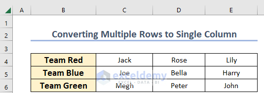
In the sample dataset, there are three rows: Team Red, Team Blue, and Team Green, with multiple columns. The goal is to convert it into a single column.
Method 1 – Using the TOCOL Function
Steps:
- Select a new cell, G5, where you want to create a single column. Here, you must keep enough cells in a column to store all the values.
- Enter the formula given below in cell G5:
=TOCOL(C4:E6)Here, in this formula, C4:E6 is the particular array that will convert into a single column.
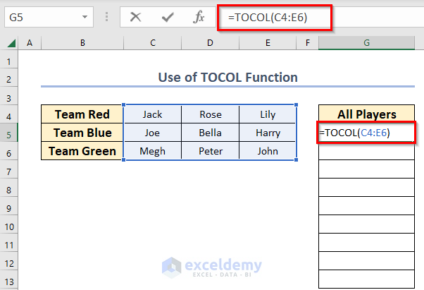
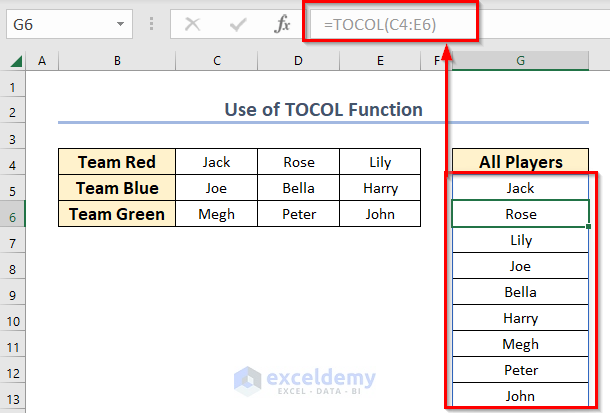
- Press ENTER.
You will get the converted column.
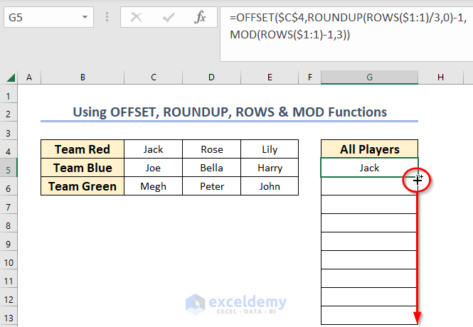
Method 2 – Using OFFSET, ROUNDUP, ROWS, and MOD Functions
Steps:
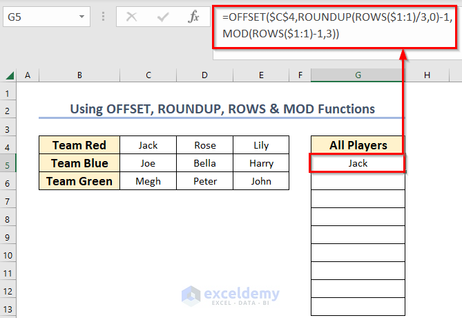
- Enter the following formula in cell G5:
=OFFSET($C$4,ROUNDUP(ROWS($1:1)/3,0)-1,MOD(ROWS($1:1)-1,3))Here, 3 is the total used column number of the dataset up to which cell the rows will convert into a column.
- Press ENTER.
Jack is placed as the first element in our desired column.
Formula Breakdown
- OFFSET: Actually, it starts from a particular cell reference, moves to a specific number of rows down, then to a specific number of columns right, and then extracts out a section from the data set having a specific height and width.
- Lastly, it returns a section from a data set with a specific height and width, situated at a specific number of rows down and a specific number of columns right from a given cell reference.
- ROUNDUP: Basically, the ROUNDUP function rounds up a number to the nearest whole number. Furthermore, it rounds up to a given number of decimal places.
- Additionally, it has two arguments. The first one is the number that we want to round up. The second one is num_digits, the place in which the position should be rounded up.
- MOD: Mainly, it gives a reminder after a number is divided by the divisor.
- Here, MOD is used to highlight an entire cell.
- ROWS: Actually, it returns the row number of a reference. So, if there are multiple references, then it returns all the rows in which those cells are located.
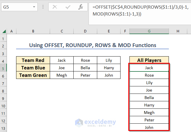
- Drag the Fill Handle icon (+ Sign) across the column until you get the last value of the last column.
It will look like this.
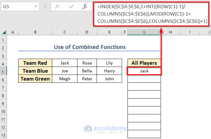
Method 3 – Combining INDEX, INT, ROW, COLUMNS, and MOD Functions
Steps:
- Enter the following formula in cell G5:
=INDEX($C$4:$E$6,1+INT((ROW(C1)-1)/COLUMNS($C$4:$E$6)),MOD(ROW(C1)-1+COLUMNS($C$4:$E$6),COLUMNS($C$4:$E$6))+1)- Press ENTER.
The value of cell C4 in G5.
Formula Breakdown
- COLUMNS: Actually, it returns the number of columns in a given range.
- Here, COLUMNS ($C$4:$E$6) returns 3 because there are 3 columns in that range.
- ROW: Mainly, this function returns the number of rows from a given reference.
- Here, ROW(C1) turns into 1.
- INT: Actually, it returns the integer portion of a number.
- So, INT({1}-1)/3) gives 0.
- MOD: Here, it gives a reminder after a number is divided by the divisor.
- Therefore, MOD({1}-1+3,3) turns into 0.
- INDEX: Basically, it returns the value at a given location of an array or range of cells.
- Lastly, INDEX($C$4:$E$6,1+{0},{0}+1) gives Jack as output.
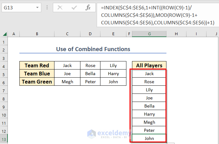
- Drag the Fill Handle icon across the column until you get the last value of the last column.
You will get the converted column.
Method 4 – Merging FILTERXML & TEXTJOIN Functions
Steps:
- Select a new cell (G5) where you want to create a single column. Here, you must keep enough cells in a column to store all the values.
- Enter the formula given below in cell G5:
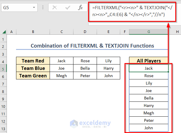
=FILTERXML("<r><n>" & TEXTJOIN("</n><n>",,C4:E6) & "</n></r>","//n")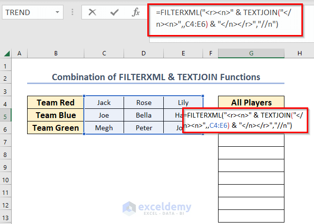
Formula Breakdown
- Here, the TEXTJOIN function will join some defined text using a delimiter. Where the delimiter is “</n><n>” and the text range is C4:E6.
- So, TEXTJOIN(“</n><n>”,,C4:E6) returns “Jack</n><n>Rose</n><n>Lily</n><n>Joe</n><n>Bella</n><n>Harry</n><n>Megh</n><n>Peter</n><n>John”
- Then, the FILTERXML function gives certain data from XML content with the help of a defined path.
- Lastly, it converts that row into a column.
- Press ENTER to get the result.
Read More: Convert Multiple Rows to Single Row in Excel
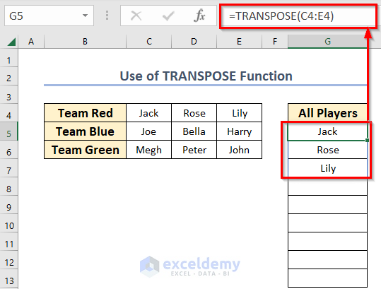
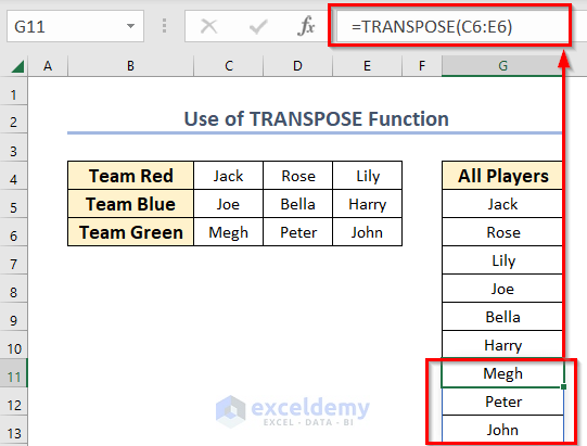
Method 5 – Using the TRANSPOSE Function
Steps:
- Select a new cell (G5) where you want to create a single column. Here, you must keep enough cells in a column to store all the values.
- Enter the following formula in cell G5:
=TRANSPOSE(C4:E4)Here, in this formula, C4:E4 is the particular row that will convert into a single column.
- Press ENTER.
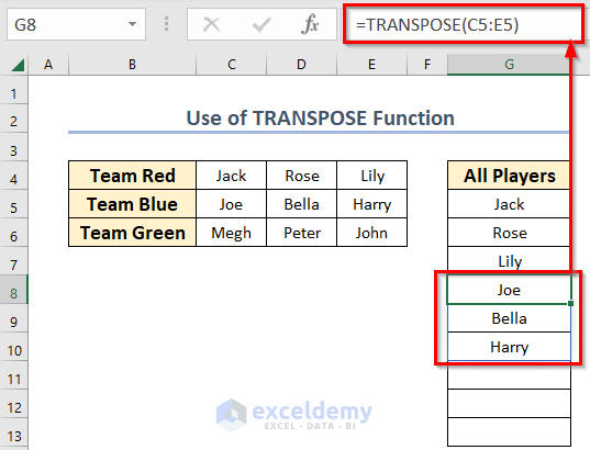
- Enter the following formula in cell G8:
=TRANSPOSE(C5:E5)In this formula, C5:E5 is the row that will convert into a single column.
- Press ENTER.
- Enter the following formula in cell G11:
=TRANSPOSE(C6:E6)Here, C6:E6 is the row that will convert into a single column.
- Press ENTER to get the final result.
Read More: How to Combine Multiple Rows into One Cell in Excel
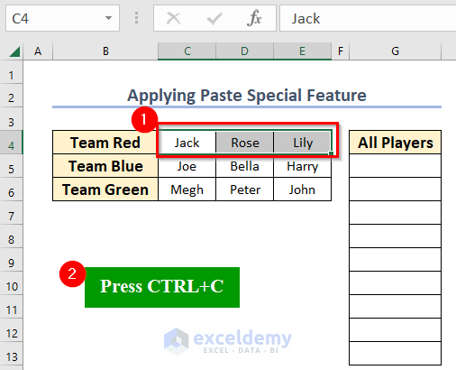
Method 6 – Using the Paste Special Feature
Steps:
- Select the 1st row (C4:E4).
- Press CTRL+C to copy the values.
- Go to cell G5 and right-click.
- From the Context Menu Bar >> choose Transpose (T) under Paste Options.
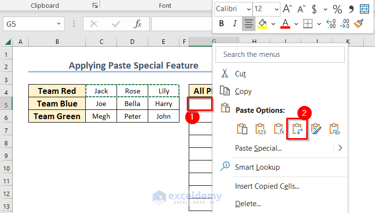
You will see the transposed column.

- Do this for the other rows.
You will get that converted column.

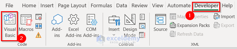
Method 7 – Using Excel VBA Code
Steps:
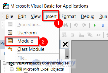
- Choose the Developer tab >> select Visual Basic.
- From the Insert tab >> select Module.
- Enter the following Code in the Module:
Sub Convert_Multi_Rows_To_A_Column()
Dim my_1st_Range As Range, my_2nd_Range As Range, my_Range As Range
Dim my_row_index As Integer
xTitleId = "Range Selection"
Set my_1st_Range = Application.Selection
Set my_1st_Range = Application.InputBox("Select Multiple Rows", xTitleId, my_1st_Range.Address, Type:=8)
Set my_2nd_Range = Application.InputBox("Select a Cell for Output", xTitleId, Type:=8)
my_row_index = 0
Application.ScreenUpdating = False
For Each my_Range In my_1st_Range.Rows
    my_Range.Copy
    my_2nd_Range.Offset(my_row_index, 0).PasteSpecial Paste:=xlPasteAll, Transpose:=True
    my_row_index = my_row_index + my_Range.Columns.Count
Next
Application.CutCopyMode = False
Application.ScreenUpdating = True
End Sub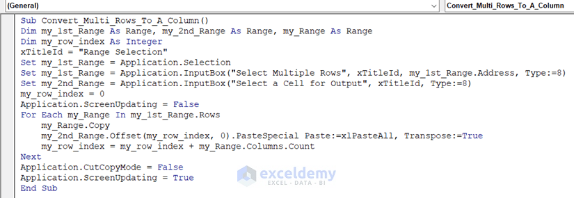
Code Breakdown
- Here, we have created a Sub Procedure named Convert_Multi_Rows_To_A_Column.
- Next, declare some variables my_1st_Range, my_2nd_Range, and my_Range as Range; my_row_index as Integer.
- Furthermore, I have used an input box named Range Selection. With the help of this box, you can choose your rows and output cell.
- After that, I used a For Each Loop to convert all the rows into a single column.
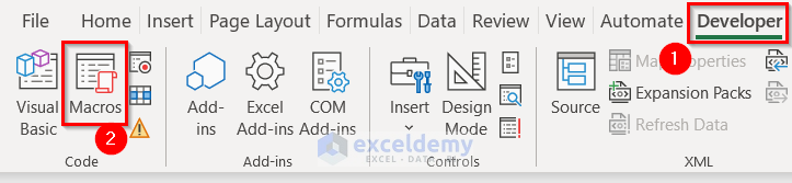
- Save the code. Go back to the Excel File.
- Fom the Developer tab >> select Macros.
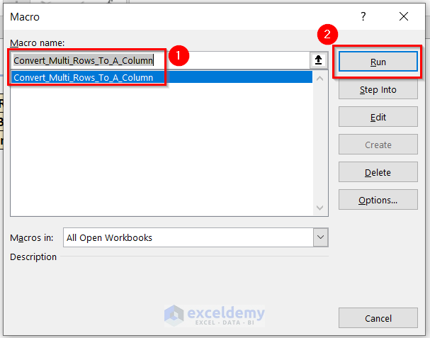
- Select the Macro name (Convert_Multi_Rows_To_A_Column) and click on Run.
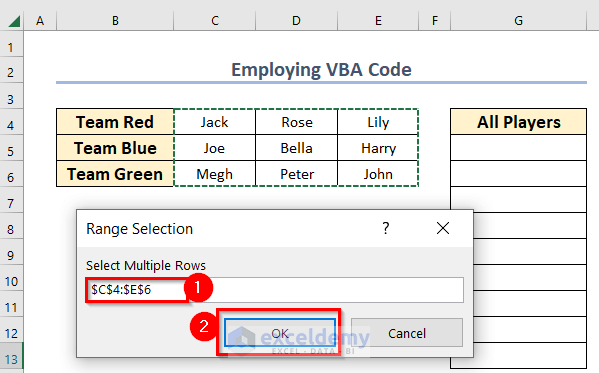
You will see the Range Selection box.
- Choose your rows in the Select Multiple Rows box.
- Press OK.
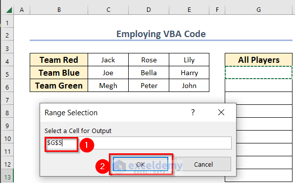
- Select a cell for output.
- Press OK.
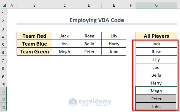
You will get your converted column.
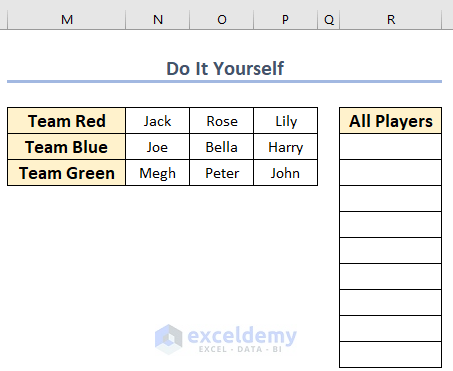
Practice Section
Now, you can practice the explained methods.
Download the Practice Workbook
You can download the practice workbook from here:
Related Articles
- How to Merge Rows and Columns in Excel
- Excel Combine Rows with Same ID
- How to Merge Rows with Comma in Excel
- How to Merge Rows Based on Criteria in Excel
- How to Merge Rows with Same Value in Excel
- How to Merge Rows Without Losing Data in Excel
- How to Merge Two Rows in Excel
<< Go Back to Merge Rows in Excel | Merge in Excel | Learn Excel
Get FREE Advanced Excel Exercises with Solutions!

Just what I needed, thanks so much! I’m still trying to get my head round the ‘Roundup’ and ‘MOD’ element of the offset formula but I managed to manipulate your formula for my data and it worked perfectly.
⇒OFFSET($B$2,ROUNDUP(ROWS($1:1)/3,0)-1,MOD(ROWS($1:1)-1,3)) : In the OFFSET formula, you need to put the cell reference, rows and cols number.
⇒OFFSET($B$2………): Here $B$2 is the cell reference of the OFFSET function.
⇒OFFSET($B$2, ROUNDUP(ROWS($1:1)/3,0)-1……): Here, the ROUNDUP function gives the specific number of rows down. ROWS function provides the number of rows in a given array. Here, the cell reference is $1:1. So, the Rows function returns 1. As we have three rows in our dataset. So, divide the return value of the Rows function by 3. It will return 0.333. Then, the ROUNDUP value will round the number into the nearest whole number. The whole number of 0.333 is 1. After that, subtract 1 from it. So, the final value is 0 which is the required rows down.
⇒OFFSET($B$2,ROUNDUP(ROWS($1:1)/3,0)-1,MOD(ROWS($1:1)-1,3)): To extract the columns right, we utilize the MOD function. It gives a reminder after a number is divided by the divisor. First, the Rows function provides the number of rows from the given array. Here, it returns 1. Then, subtract 1 from the return value. Then, divide the value by the total number of columns. The MOD function will return the reminder. Here, it returns 0.
So, for cell reference $B$2 and rows 0 down and cols 0 right, it returns Arif as our answer. Do the same for other cases.
Try this solution I think you will get your desired result. If you face any more problems, inform us.