How to Combine Multiple Rows in One Cell in Excel: 6 Simple Methods
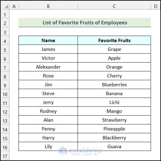
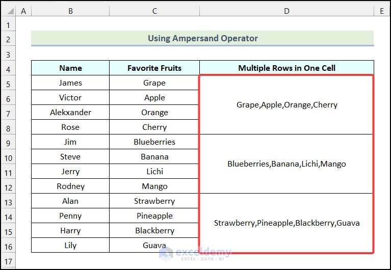
We have the List of Favorite Fruits of Employees as our dataset. We have two columns for Name and Favorite Fruits. We’ll combine multiple rows in one cell.
Method 1 – Using the Ampersand Operator
Steps:
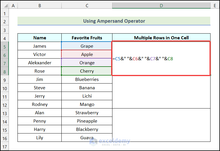
- Use the following formula in cell D5.
=C5&" "&C6&" "&C7&" "&C8Cells C5, C6, C7, and C8 indicate the first four cells of the Favorite Fruits columns.
- Hit Enter.
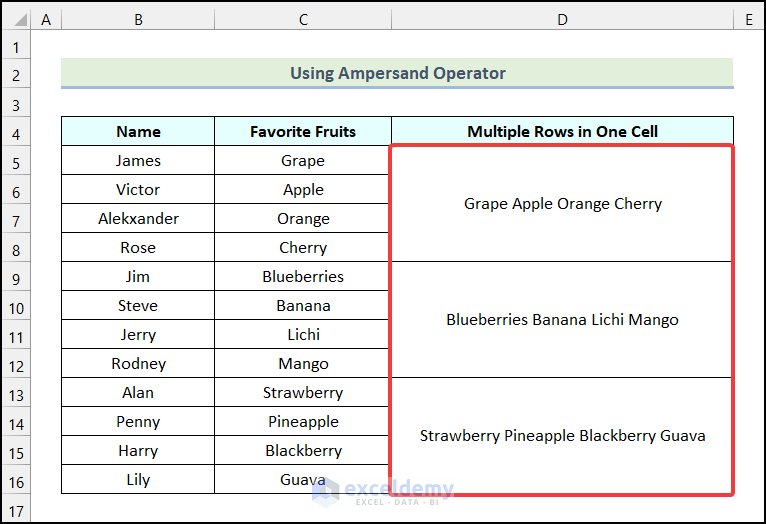
You will get the first four cells of the Favorite Fruits column combined in cell D5 as shown in the following image.

- Use Excel’s AutoFill feature to obtain the remaining outputs.
If you want to separate your row’s content using comma (,), space, or any character, insert those signs between the double quote (“ ”).
- Here’s an example of using the comma delimiter:
=C5&","&C6&","&C7&","&C8
- Here, each cell is separated by a comma.
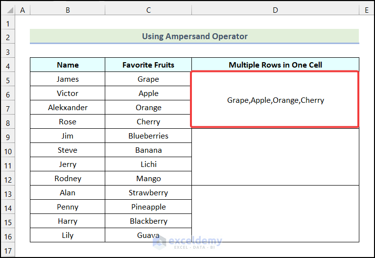
- Use Excel’s AutoFill option to get the combined list for the rest of the cells as demonstrated in the image below.
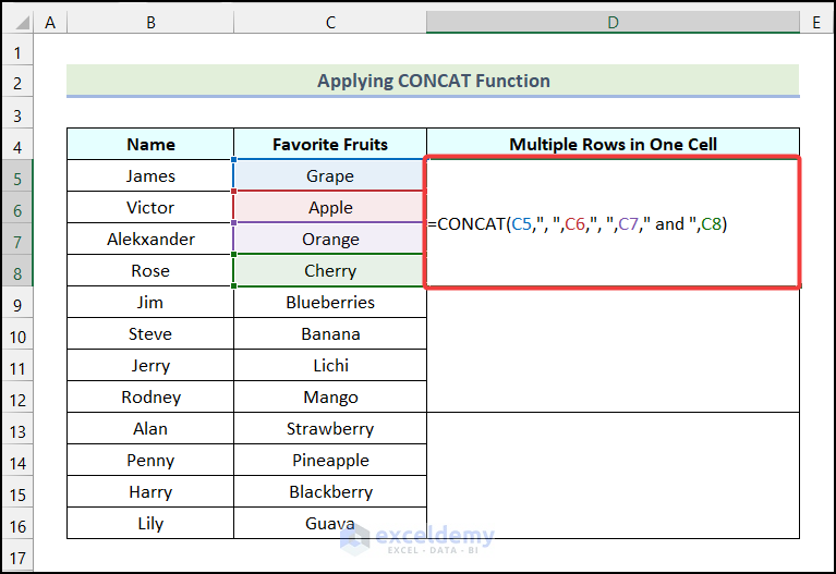
Method 2 – Applying the CONCAT Function
Steps:
- Apply the following formula in cell D5.
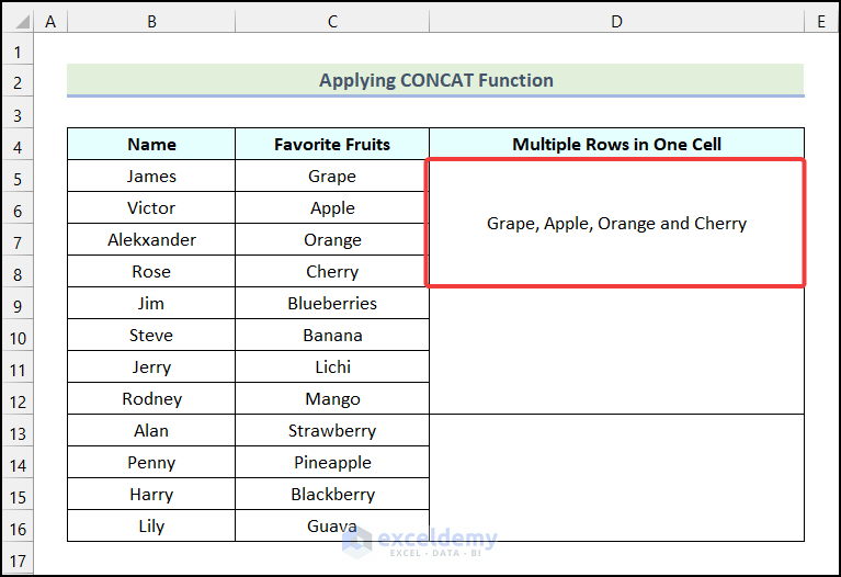
=CONCAT(C5,", ",C6,", ",C7," and ",C8)- Hit Enter.
- You will get the following output.
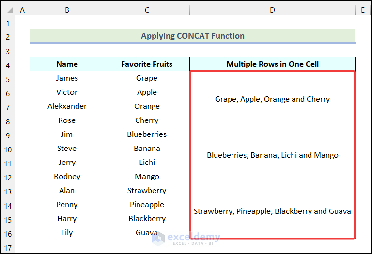
- Apply Excel’s AutoFill feature to get the combined list of Favorite Fruits for the remaining cells.
Read More: How to Merge Two Rows in Excel
Method 3 – Utilizing CONCATENATE and TRANSPOSE Functions
Steps:
- Select the cell where you want to put your combined data.
- Insert the following formula.
=TRANSPOSE(C5:C8)- Press the F9 key.
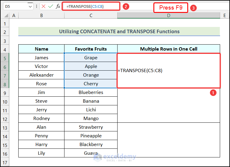
- The row values within curly braces as marked in the following picture.
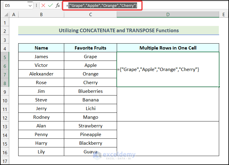
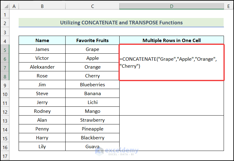
- Remove the curly braces and wrap the list in a CONCATENATE function:
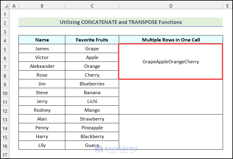
=CONCATENATE("Grape","Apple","Orange","Cherry")- Hit Enter.
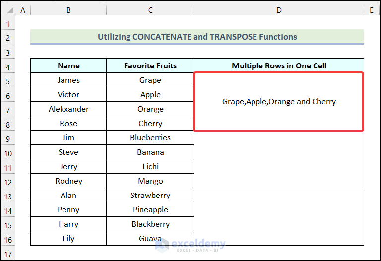
- You will get the following output on your worksheet.
- You can use delimiters between the values:
=CONCATENATE("Grape",",","Apple",",","Orange"," and ","Cherry")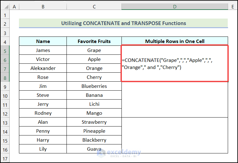
A comma will be added between the texts and the “and” separator will be added before the last text as demonstrated in the following image.
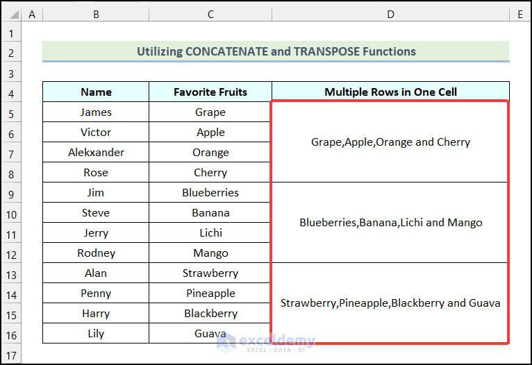
- Use Excel’s AutoFill feature to get the rest of the outputs.
Method 4 – Implementing the TEXTJOIN Function
Steps:
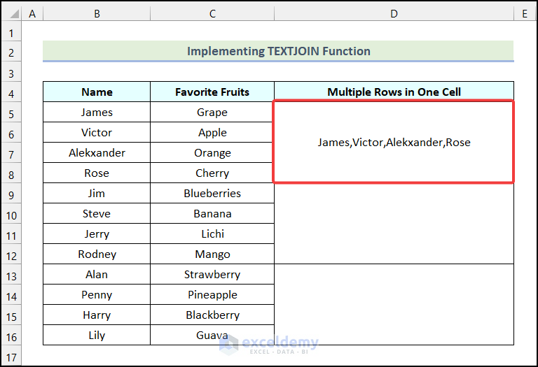
- Use the following formula in cell D5.
=TEXTJOIN(",",TRUE,B5:B8)- Hit Enter.
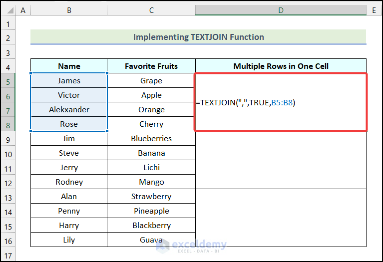
- You will get the combined list of the first four cells of the Favorite Fruits column in cell D5. We used a comma (,) as a delimiter.
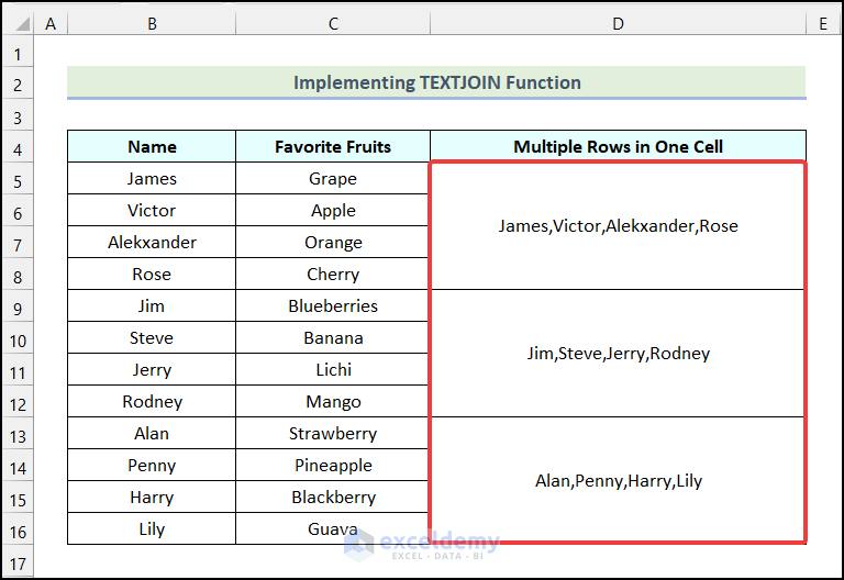
- Use Excel’s AutoFill option to obtain the remaining outputs as shown in the image below.
Method 5 – Using the Formula Bar
Steps:
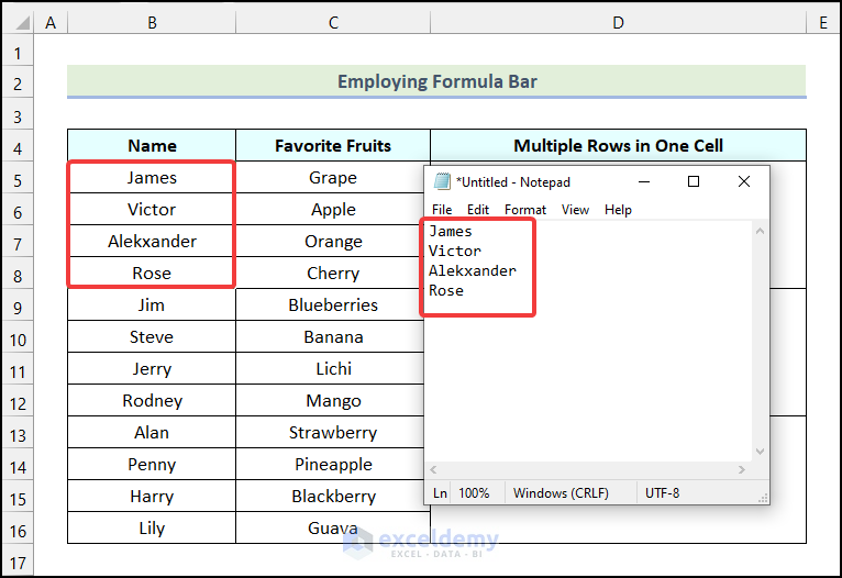
- Select the cells you want to combine and press Ctrl + C to copy the cells.
- Open Notepad on your computer.
- Press the keyboard shortcut Ctrl + V to paste the cells into Notepad.
- Select the values and press Ctrl + C to copy them.
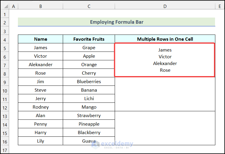
- Select the cell where you want to show the combined list of Names. We selected the cell D5.
- Go to the Formula Bar and press Ctrl + V to paste the copied Names from the Notepad.
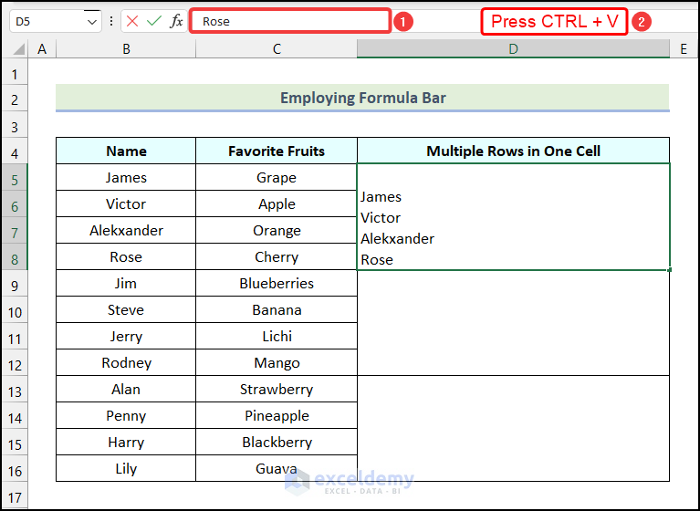
- You will get the list of Names combined in cell D5.
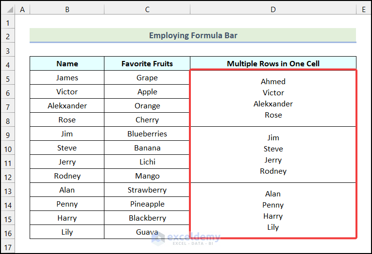
- Follow the same steps to get the remaining outputs as shown in the following image.
Method 6 – Incorporating VBA Macro
Steps:
- Go to the Developer tab.
- Select the Visual Basic option from the Code group.
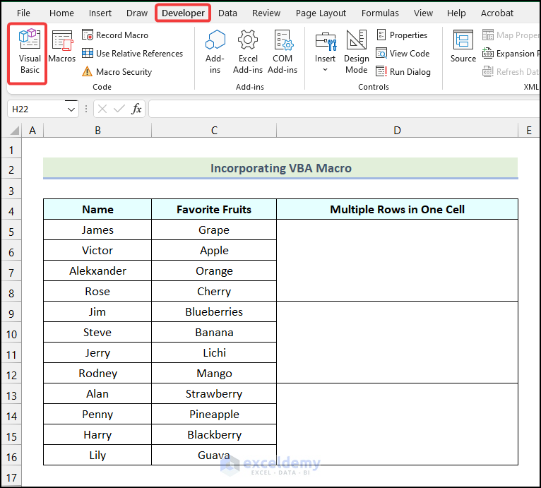
The Microsoft Visual Basic for Applications window will appear on your worksheet.

- Go to the Insert tab.
- Choose the Module option from the drop-down.
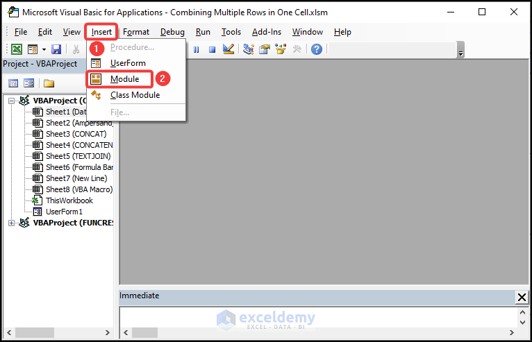
- Insert the following code in the newly created Module1.
Sub Multiple_Rows_into_One_Cell()
Dim i As Integer
If Selection.Cells.Count > 1 Then
For i = 1 To Selection.Cells.Count
Cells(ActiveCell.Row, 4).Value = Cells(ActiveCell.Row, 4).Value _
& " " & Selection.Cells(i).Value
Next i
End If
End Sub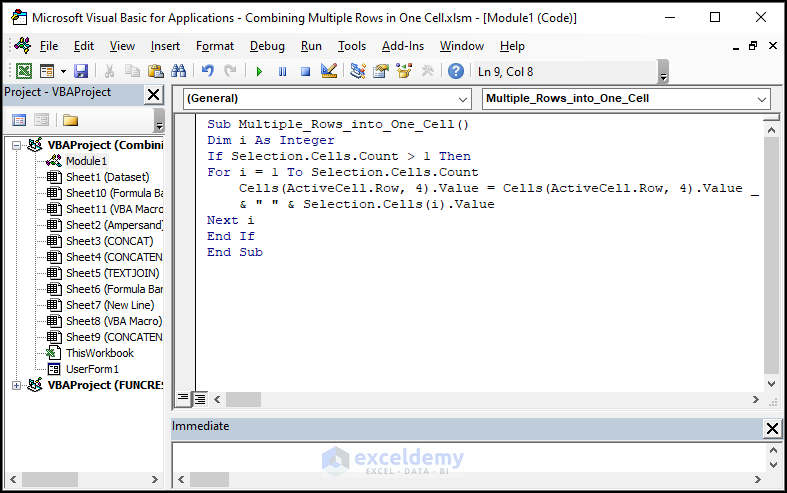
Code Breakdown
- We initiated a sub-procedure named Multiple_Rows_into_One_Cell.
- We used the IF statement to check whether the count selected is greater than 1.
- We used a For Next loop to assign the combined list of the selected cells in cell D5.
- We used Space as a separator.
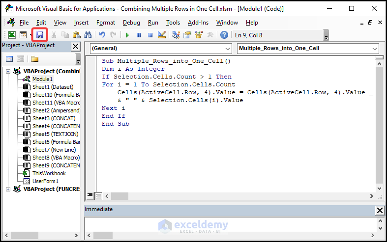
- Click on the Save option.
- Press the keyboard shortcut Alt + F11 to return to the worksheet.
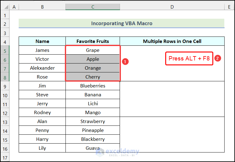
- Select the cells you want to combine. We selected cells C5:C8.
- Use the keyboard shortcut Alt+ F8 to open the Macro window.
The Macro dialog box will open on your worksheet as shown in the following image.
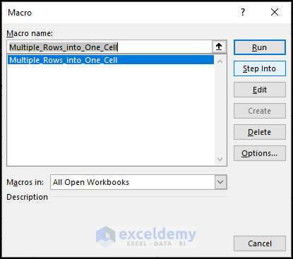
- Select the Multiple_Rows_into_One_Cell option.
- Click on the Run option.

- You will get the combined list of your selected cells in cell D5.
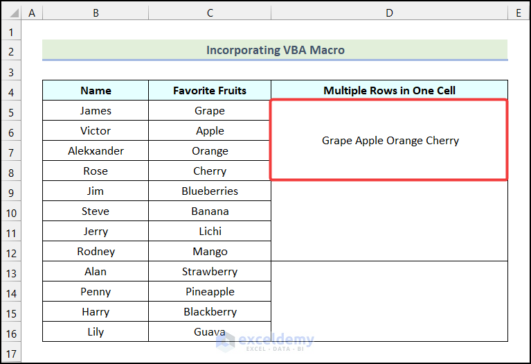
- Follow the same steps for the rest of the cells and you will get the following output as demonstrated in the following picture.

How to Insert a New Line Within a Cell in Excel
Steps:
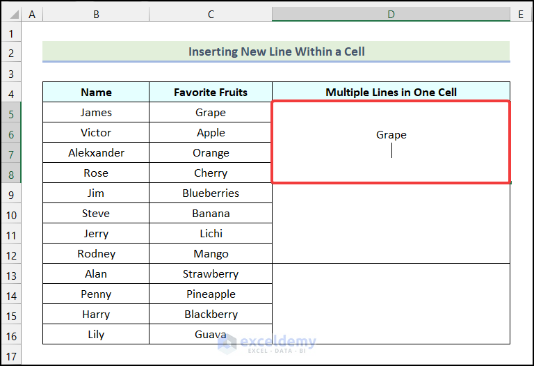
- Type in the first cell of the Favorite Fruits column as shown in the image below.
- Use the keyboard shortcut Alt + Enter to insert a new line.
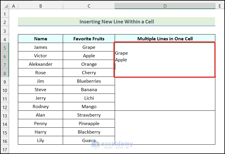
- Type in the second value of the Favorite Fruits column and then press Alt + Enter.
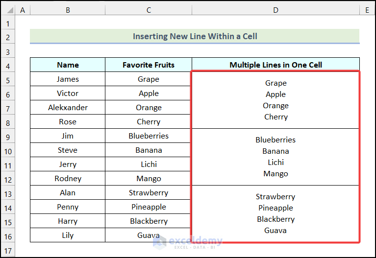
- Repeat the process and you will get the following output.
Practice Section
We have provided a Practice Section on the right side of the worksheet.
Download the Practice Workbook
Further Readings
- How to Combine Rows with Same ID in Excel
- How to Merge Rows in Excel Based on Criteria
- Excel Merge Rows with Same Value
- How to Merge Rows Without Losing Data in Excel
- How to Merge Rows with Comma in Excel
- How to Merge Rows and Columns in Excel
- How to Convert Multiple Rows to a Single Column in Excel
- How to Convert Multiple Rows to Single Row in Excel
<< Go Back to Merge Rows in Excel | Merge in Excel | Learn Excel
Get FREE Advanced Excel Exercises with Solutions!
