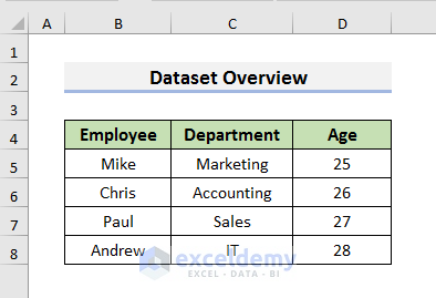
How to Merge Rows with Commas in Excel (4 Methods)

Dataset Overview

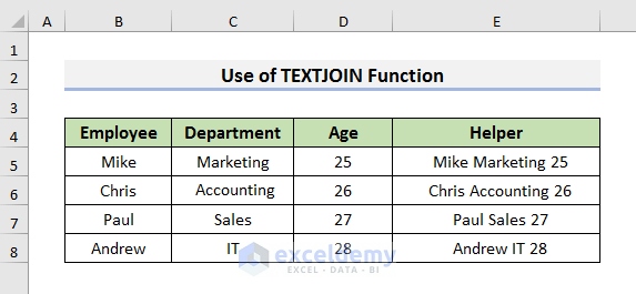
To explain the methods, we will use a dataset that contains information about the Department and the Age of some employees of a company.

Method 1- Using Excel Functions

1.1 Using the CONCATENATE Function

The CONCATENATE function allows us to combine cell values. Follow these steps:

Create a Helper column.
In cell E5, enter the formula:

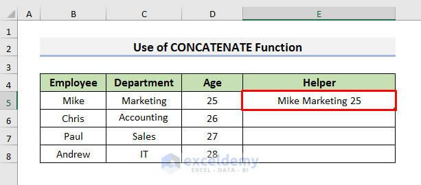
=CONCATENATE(B5," ",C5," ",D5)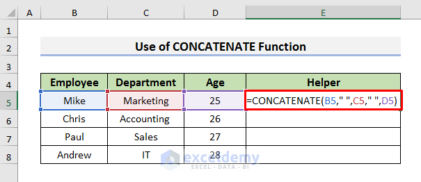

Press Enter to see the result.

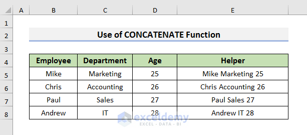
Drag the Fill Handle down to apply the formula to the remaining cells.

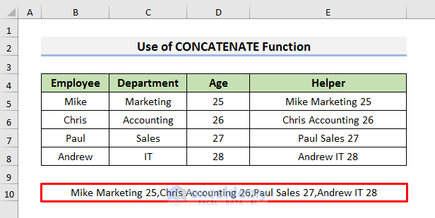
In an empty cell, insert the formula:

=CONCATENATE(E5,",",E6,",",E7,",",E8)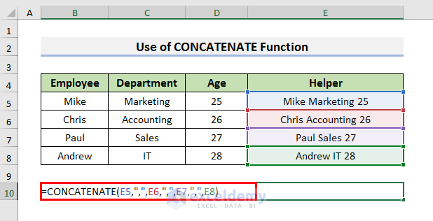

Press Enter. This will display the merged rows with commas.

1.2 Using the TEXTJOIN Function

The TEXTJOIN function combines text from different cells. Here’s how:

Create another Helper column.
In cell E5, enter the formula:

=TEXTJOIN(" ",TRUE,B5:D5)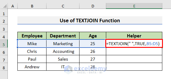

Press Enter to see the result.

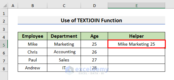
Drag down the Fill Handle to apply the formula to other cells.

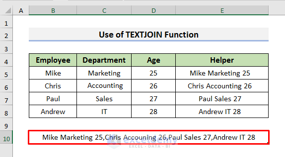
In cell B10, use the formula:

=TEXTJOIN(",",TRUE,E5:E8)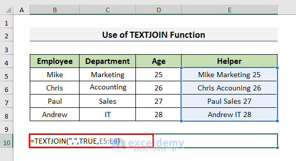

Press Enter. This will give you the merged rows with commas.

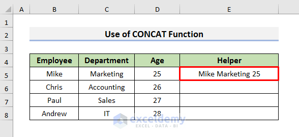
1.3 Using the CONCAT Function

The CONCAT function is similar to CONCATENATE and can also merge cell values. Follow these steps:

Create yet another Helper column.
In cell E5, enter the formula:

=CONCAT(B5," ",C5," ",D5)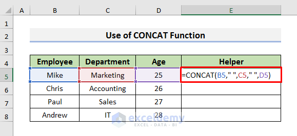

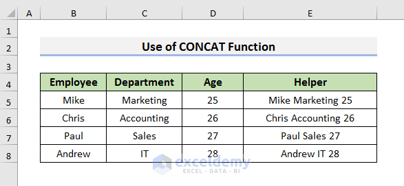
Press Enter to see the result.

Drag the Fill Handle down to autofill the formula.

In an empty cell, insert the formula:

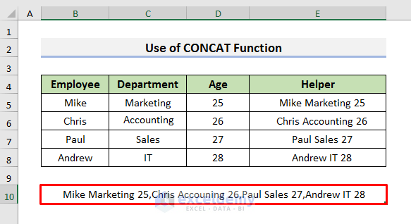
=CONCAT(E5,",",E6,",",E7,",",E8)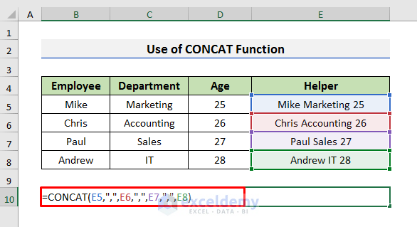

Press Enter. This will display the merged rows with commas.

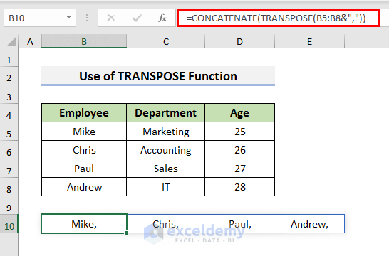
1.4 Using TRANSPOSE and CONCATENATE

Combine the TRANSPOSE and CONCATENATE functions:

Select Cell B10.
Enter the formula:

=CONCATENATE(TRANSPOSE(B5:B8&","))

This will convert the first value from each row in Column B into a single row with comma separators.

Press Enter to see results like the picture below.

To show the Department and Age, enter the formula:

=CONCATENATE(TRANSPOSE(B5:D8&","))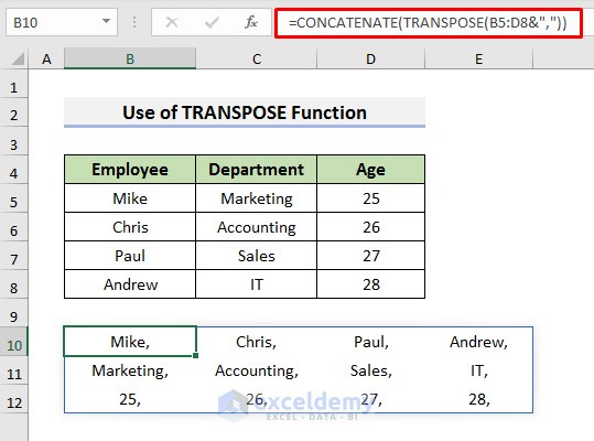

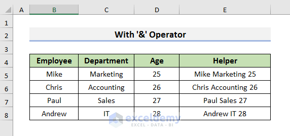
Method 2 – Merge Rows in Excel Using the Ampersand (&) Operator

In this method, we’ll explore how to merge rows in Excel using the Ampersand (&) operator. We’ll continue using the same dataset to illustrate the process. Let’s dive into the steps:

Create a Helper column to merge the cells within each row.
Select cell E5.
Enter the formula:

=B5&" "&C5&" "&D5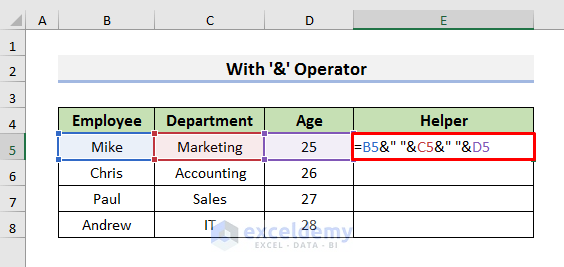

Press Enter to see the result.

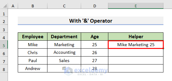
Autofill the formula down to apply it to the remaining cells.

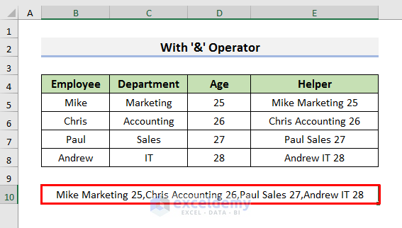
In an empty cell, use the formula:

=E5&","&E6&","&E7&","&E8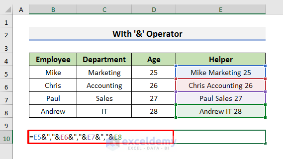

Press Enter to display the merged rows with commas.

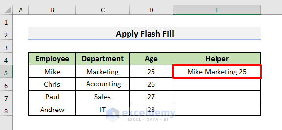
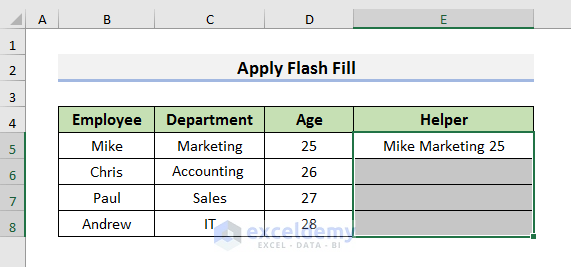
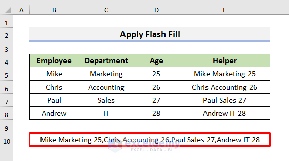
Method 3 – Excel Flash Fill

The Flash Fill feature in Excel allows us to quickly merge rows with a specific pattern. Follow these steps:

Select cell E5.
Enter the values from cells B5, C5, and D5 with spaces (as shown in the picture).

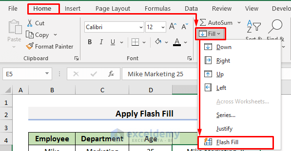
Select the cells you want to fill (starting from E5).

Go to the Home tab and choose Fill from the drop-down menu.
Select Flash Fill.

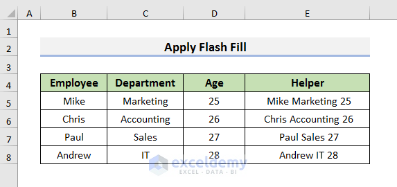
The results will automatically populate (see picture).

Select Cell B10 and enter the formula:

=CONCAT(E5,",",E6,",",E7,",",E8)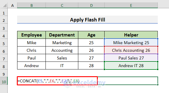

Press Enter to see the merged rows with commas.

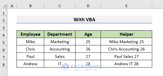
Method 4 – Using VBA (Visual Basic for Applications)

In this method, we’ll create a user-defined function using VBA to join rows with a comma separator. Follow these steps:

Select cell E5 and enter the formula:

=CONCAT(B5,",",C5,",",D5)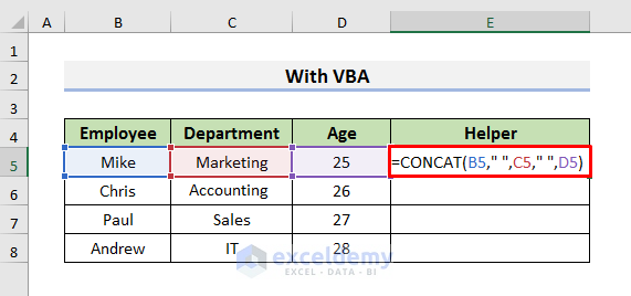

Press Enter and drag the Fill Handle down to apply the formula.

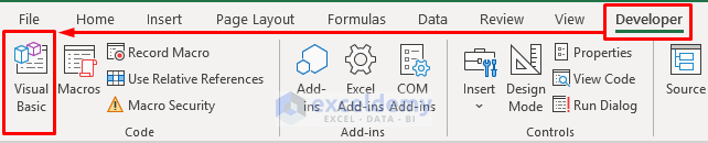
Go to the Developer tab and select Visual Basic to open the Visual Basic window.

Click Insert and choose Module to open the Module window.
Enter the following code in the Module window:

Function Merge(xWorkRg As Range, Optional Sign As String = ",") As String
Dim xRg As Range
Dim xOutSr As String
For Each xRg In xWorkRg
If xRg.Text <> " " Then
xOutSr = xOutSr & xRg.Text & Sign
End If
Next
Merge = Left(xOutSr, Len(xOutSr) - 1)
End Function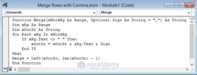

Press Ctrl+S to save the code.
Close the Visual Basic window.
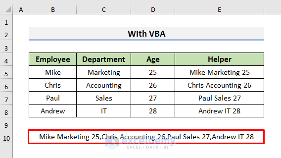
Enter the following formula in Cell B10:

=Merge(E5:E8)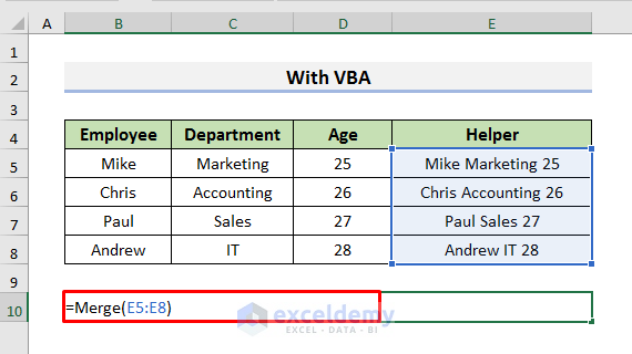

Press Enter to see the merged result.

Things to Remember

These methods work for merging rows with values in multiple columns.
For merging rows in a single column, adjust the cell positions accordingly.
To use a different separator, replace the comma in the formula with your desired separator.

Download Practice Book

You can download the practice workbook from here:

Merge Rows with Comma.xlsm

<< Go Back to Merge Rows in Excel | Merge in Excel | Learn Excel

Get FREE Advanced Excel Exercises with Solutions!

2 Comments

Biplab Das Jun 21, 2022 at 8:39 AM

Have any idea about VBA or Formula Without Helper Column ?
- Reply
  Mursalin Jul 19, 2022 at 2:04 PM
  
  Hi BIPLAB,
  Thanks for your query. You can build a formula with the nested CONCAT function. In that case, you don’t need any helper column. For the dataset we have discussed in the article, the formula will be:
  =CONCAT(CONCAT(B5,” “,C5,” “,D5),”,”, CONCAT(B6,” “,C6,” “,D6),”,”,CONCAT(B7,” “,C7,” “,D7),”,”,CONCAT(B8,” “,C8,” “,D8))
  You can also use the VBA code below. To apply this, you need to select the rows of the first column of the dataset and then run the code from the Macro window.
  
  Sub Merge_Rows_with_Comma()
  
  Dim iSelection As Range
  Dim iRow As Range
  Dim iCell As Range
  Dim iStr As String
  
  Application.ScreenUpdating = False
  On Error Resume Next
  Set iSelection = Intersect(Selection, ActiveSheet.UsedRange)
  
  For Each iRow In iSelection.Rows
  For Each iCell In iRow.Cells
  iStr = iStr & ” ” & VBA.Trim$(iCell)
  Next iCell
  iRow.ClearContents
  iRow.Cells(1, 1).NumberFormat = “@”
  iRow.Cells(1, 1) = Mid(iStr, 2)
  iStr = vbNullString
  Next iRow
  
  For Each iCell In iSelection
  iStr = iStr & “,” & VBA.Trim$(iCell)
  Next
  
  With ActiveWindow
  .Selection.ClearContents
  .Selection(1, 1).NumberFormat = “@”
  .Selection(1, 1).Value = Mid(iStr, 2)
  End With
  End Sub