While working in Excel, sometimes we need to merge two columns into a single one. Along with it, we also need to remove the duplicate one as well. To perform these tasks, Excel has benefitted us with some effective methods. In this article, we will discuss how to merge two columns in Excel and remove duplicates with 6 effective methods.
How to Merge Two Columns in Excel and Remove Duplicates: 5 Effective Methods
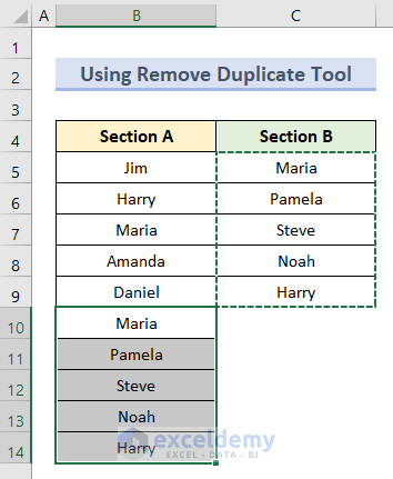
Let us take an example for discussion. Here, the dataset shows the information on the student list of 2 sections in a class.

Now, we will follow the methods below to merge these two columns. Also, we will remove the duplicate data.
Method 1: Use Remove Duplicate Tool to Merge Columns Without Duplicates
The use of the Remove Duplicate tool is one of the easiest methods to merge columns and remove duplicates. Follow the steps below:
- In the beginning, select cell range C5:C9.
- Then, right-click on it and click on Copy.
- Otherwise, press Ctrl + C on your keyboard.

- After this, select cell B10 and press Ctrl + V to paste the cells.
- Another way is to right-click on cell B10 and click on Paste to see the output below:
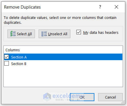
- Now, go to the Data tab and select the Remove Duplicate icon from the Data Tools group.

- Further, it will show the window.
- Here, deselect the second column and press OK.
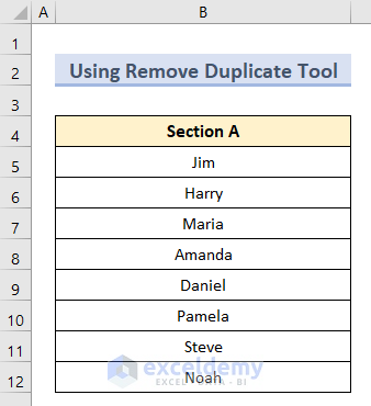
- Lastly, you will see a message box showing the result of removing duplicates.

- Finally, delete the second column and you will see this final output.
Method 2: Merge Two Columns and Remove Duplicates with Excel VBA
This second method will guide you through the process of merging two columns and removing duplicates by applying Excel VBA codes. Simply go through the process below:
- First, copy and paste the second column below the first one by pressing Ctrl + C and Ctrl + V respectively.
- Then, go to the Developer tab and select Visual Basic under the Codes group.

- Next, choose Module from the Insert section.

- Now, insert this code on the blank page.
Sub Remove_Duplicates()

  Range("B4:B14").RemoveDuplicates Columns:=1, Header:=xlYes

End Sub
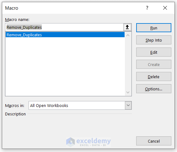
- Next, close this window and select Macros from the Developer tab.

- Lastly, click on Run in the Macro window.
- Finally, you will see that the duplicate values are removed from the list.

Method 3: Combine Two Columns in Excel with Array Formula
The Array formula is a powerful method to extract unique values from two columns. It helps to calculate multiple columns and rows at once, along with erasing the duplicate values as well. Let’s see how it works.
- Firstly, insert this formula in cell E5.
=INDIRECT(TEXT(MIN(IF(($B$5:$C$9<>"")*(COUNTIF($E$4:E4,$B$5:$C$9)=0),ROW($5:$9)*100+COLUMN($B:$C),4^5)),"R0C00"),)&""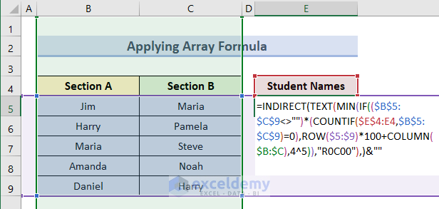
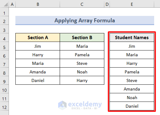
- Secondly, press Enter.
- Then, you will see the first value from the two columns.

- Lastly, use the Fill Handle tool to copy this formula in cell range E6:E12.
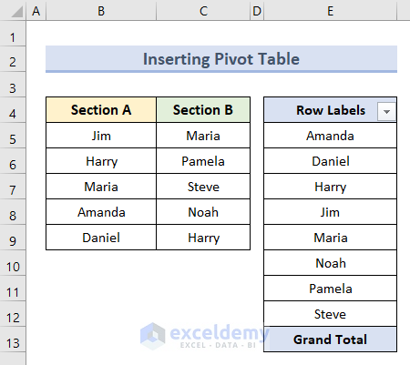
Method 4: Insert Pivot Table for Merging Columns and Removing Duplicates
Another useful technique to merge columns is to insert a Pivot Table. In parallel, it will remove the duplicate values as well. Check the steps below:
- First, insert a blank column beside the dataset.

- Then, press Alt + D and then P to open the PivotTable and PivotChart Wizard window.
- Here, apply the selections as per the image below:

- After this, press Next.
- Following, select the option Create a single page field for me and press Next.

- After that, insert the cell range B4:D9 in the Range box and click Add.
- Then, press again Next.

- Lastly, insert cell reference F4 as the location for the pivot table.
- Now, hit on Finish.

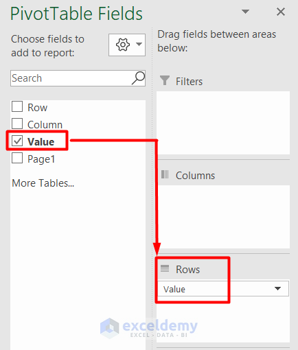
- Thereafter, you will see the new PivotTable Fields.
- Here, drag the Value field to the Rows section and deselect others.
- Finally, you will get your merged values in a pivot table removing the duplicates.
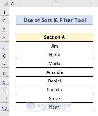
Method 5: Use Sort & Filter Tool to Merge Two Columns in Excel
This fifth method will guide you in using the Sort & Filter tool for merging both columns. It will also extract the unique values and remove the duplicate ones.
- In the beginning, copy the second column values by pressing Ctrl +C on your keyboard.
- Then, paste it by pressing Ctrl + V below the first column.
- Now, select cell range B4:B14.

- After this, go to the Data tab and select Advance under the Sort & Filter group.

- Following, keep the selections as per the image below.

- Then, press OK.
- Finally, you will get the merged column without duplicate values.
Download Practice Workbook
Download this sample file to try it by yourself.
Conclusion
Concluding the article with the hope that it was a helpful one for you on how to merge two columns in Excel and remove duplicates with 5 effective methods. Let us know if you have other solutions.
<< Go Back to Merge Columns in Excel | Merge in Excel | Learn Excel
Get FREE Advanced Excel Exercises with Solutions!
