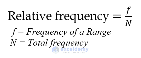
Relative Frequency
Relative frequency is the ratio of a frequency within a specific range to the total number of frequencies. The percentage or dominance of a class range over the overall range can be determined using relative frequency.
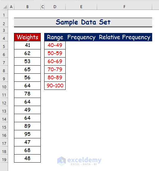
The sample dataset showcases people’s weight.
To determine the frequency of each class:
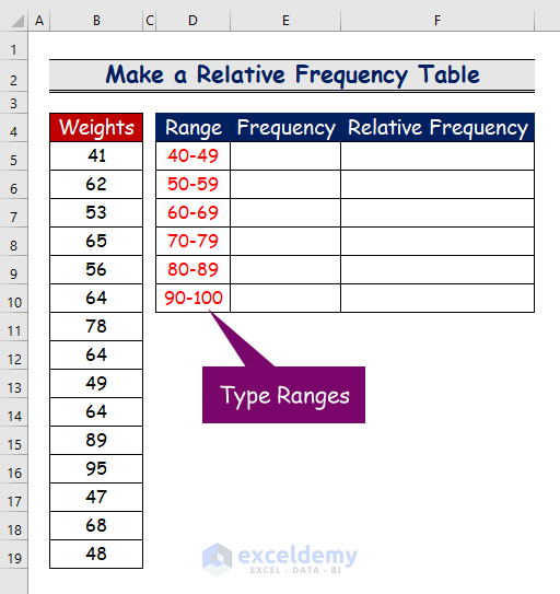
Step 1- Specify the Range of Weights
- Specify the range with an equal interval. Here, a range from 40 to 100 with an equal interval of 10.
Read More: How to Make a Categorical Frequency Table in Excel
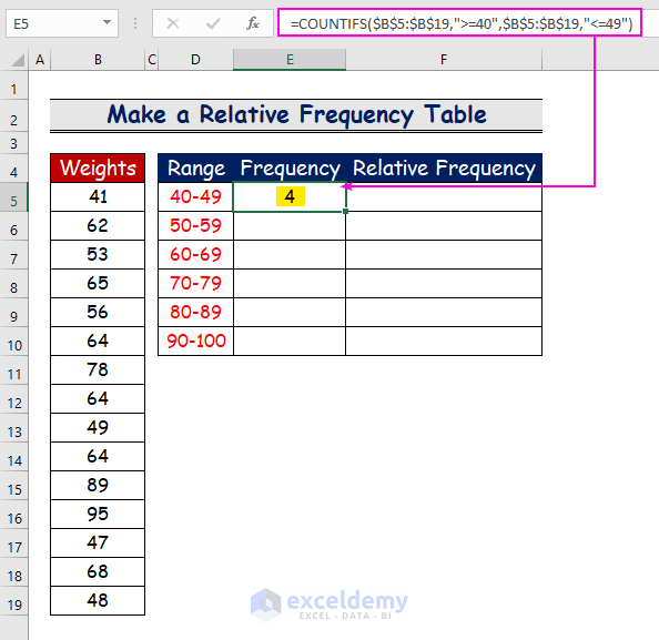
Step 2 – Use the COUNTIFS Function to Count the Frequency
To count the frequency for the range 40–49:
- In E5, use the conditions greater than or equal to 40 and less than or equal to 49 as the criteria argument:
=COUNTIFS($B$5:$B$19,">=40",$B$5:$B$19,"<=49")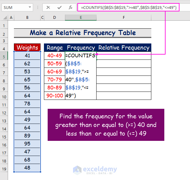
- As there are four cell values for the weight range between 40 and 49 kg, the output is 4.
- Use the same function for the other ranges. For example, in E10, use the following formula:
=COUNTIFS($B$5:$B$19,">=90",$B$5:$B$19,"<=100")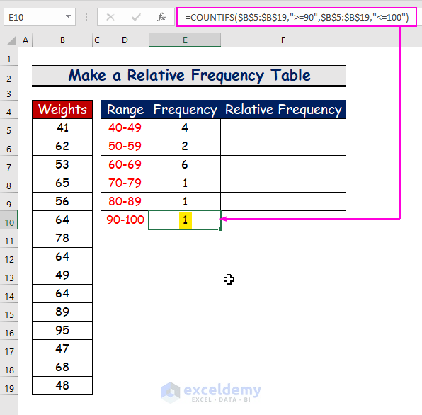
Read More: How to Make a Contingency Table in Excel
Step 3 – Use the SUM Function to Count the Total Frequency
- To count the total frequency of the dataset, enter the following formula:
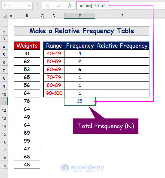
=SUM(E5:E10)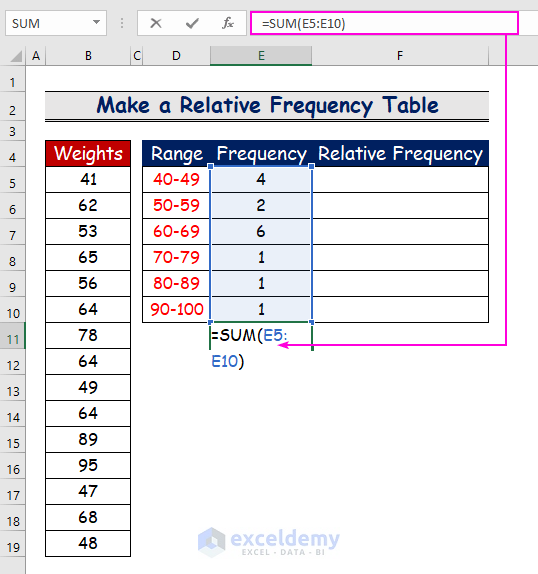
- Press Enter to see the result: 15.
Read More: How to Calculate Percent Frequency Distribution in Excel
Step 4 – Use a Formula to Create a Relative Frequency Table
- Divide the frequency of each cell by the total frequency to find the relative frequency.
- For the cell value in E5 (4), use the following formula.
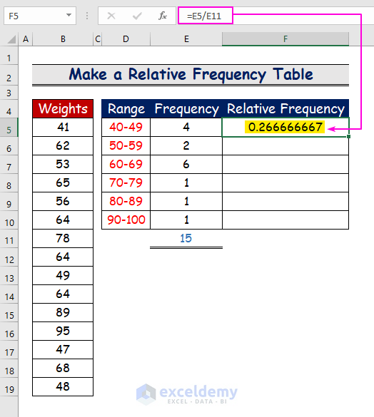
=E5/E11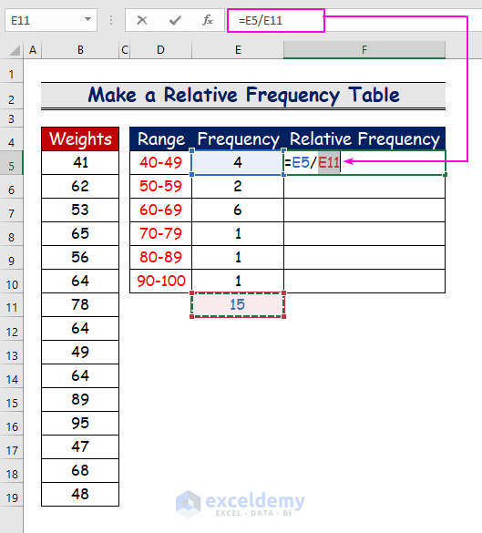
The output is 0.2666667: the relative frequency of the range 40–49.
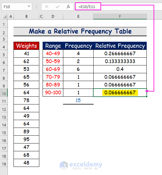
- Repeat the procedure for the other ranges.
- The relative frequency table will be displayed.
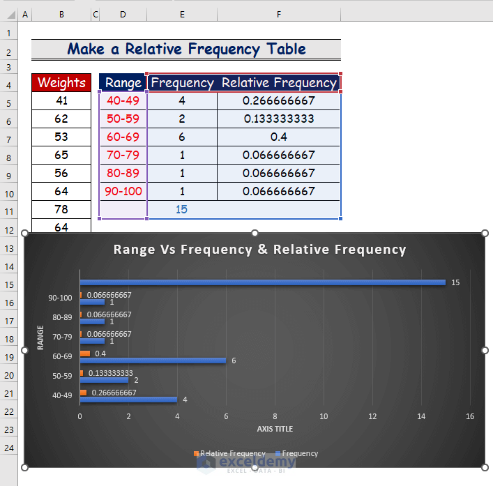
Step 5 – Insert a Chart with a Relative Frequency Table
- In the Insert tab, select a chart.
- The orange color denotes the relative frequency of a given range, whereas the blue color denotes the frequency of that specific range.
Download Practice Workbook
Related Articles
<< Go Back to Frequency Distribution in Excel | Excel for Statistics | Learn Excel
Get FREE Advanced Excel Exercises with Solutions!
