What Is a Contingency Table?
Contingency Tables are a summary of various categorical variables. Contingency Tables are also known as Cross Tabs and Two-way Tables. Generally, a Contingency Table displays the frequency distribution of several variables in a table or matrix format. It provides a quick overview of the interrelationships between the variables in the table. Contingency Tables are widely used in various research sectors.
How to Make a Contingency Table in Excel: 2 Simple Methods
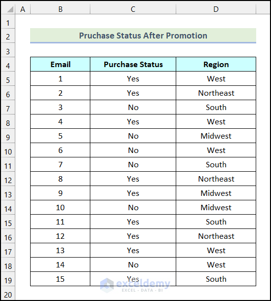
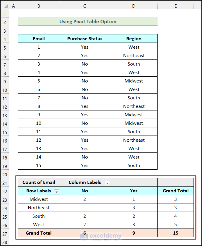
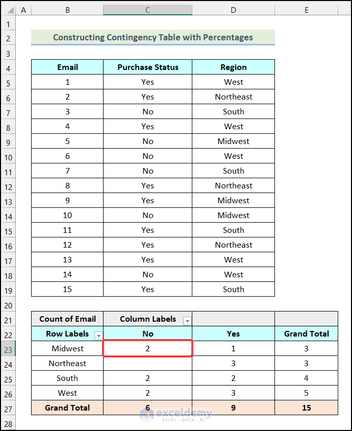
Let’s say an online retailer sent an Email about promotional discounts to potential customers of different Regions. We have the Purchase Status of some of the customers. We’ll make a Contingency Table from this data.
Method 1 – By Creating a PivotTable
Steps:
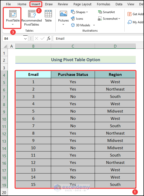
- Select the dataset and go to the Insert tab from Ribbon.
- Choose the PivotTable option from the Tables group.
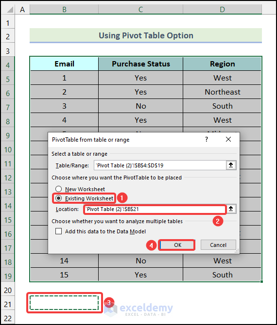
The PivotTable from table or range dialog box will open on your worksheet.
- Choose the Existing Worksheet option.
- Click on the Location field and select cell C21.
- Click OK.
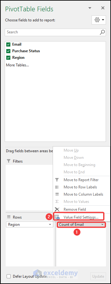
The PivotTable Fields dialog box will open.
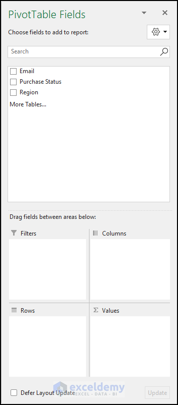
- Drag the Region option into the Rows section.
- Drag the Email option into the Values section.
- Drag the Purchase Status option into the Columns sections.
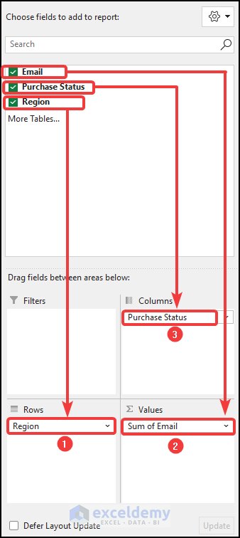
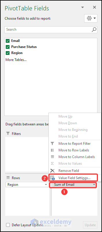
- Click on the Sum of Email as marked in the image below.
- Select the Value Field Settings option.
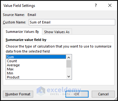
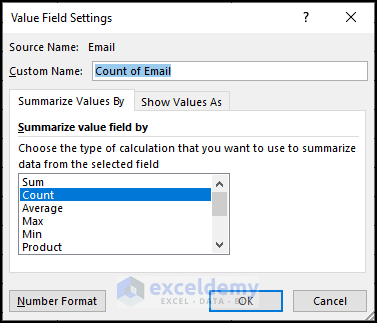
The Value Field Settings dialog box will be available on your worksheet.
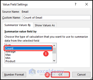
- Select the Count option.
- Click OK.
You will have a Contingency Table as demonstrated in the following picture.
Read More: How to Calculate Percent Frequency Distribution in Excel
Method 2 – Applying an Excel Formula
Steps:
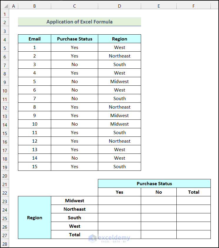
- Create a table as shown in the following picture.
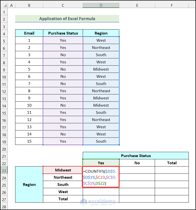
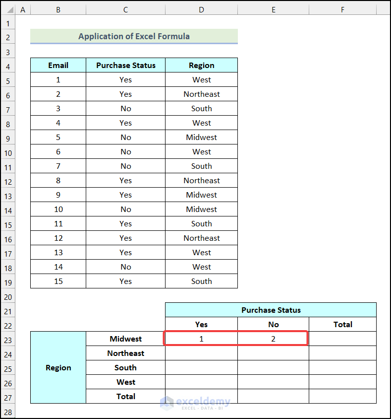
- Enter the following formula in cell D23.
=COUNTIFS($D$5:$D$19,$C23,$C$5:$C$19,D$22)The range of cells $D$5:$D$19 indicates the cells of the Region column, cell C23 represents the selected Region, the range of cells $C$5:$C$19 refers to the cells of the Purchase Status column, and cell D22 indicates the selected Purchase Status.
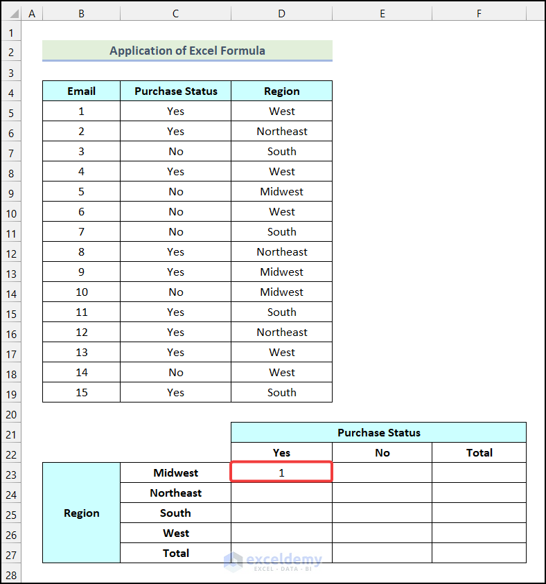
- Press Enter.
You will know how many customers in the Midwest region purchased after receiving the promotional Email.
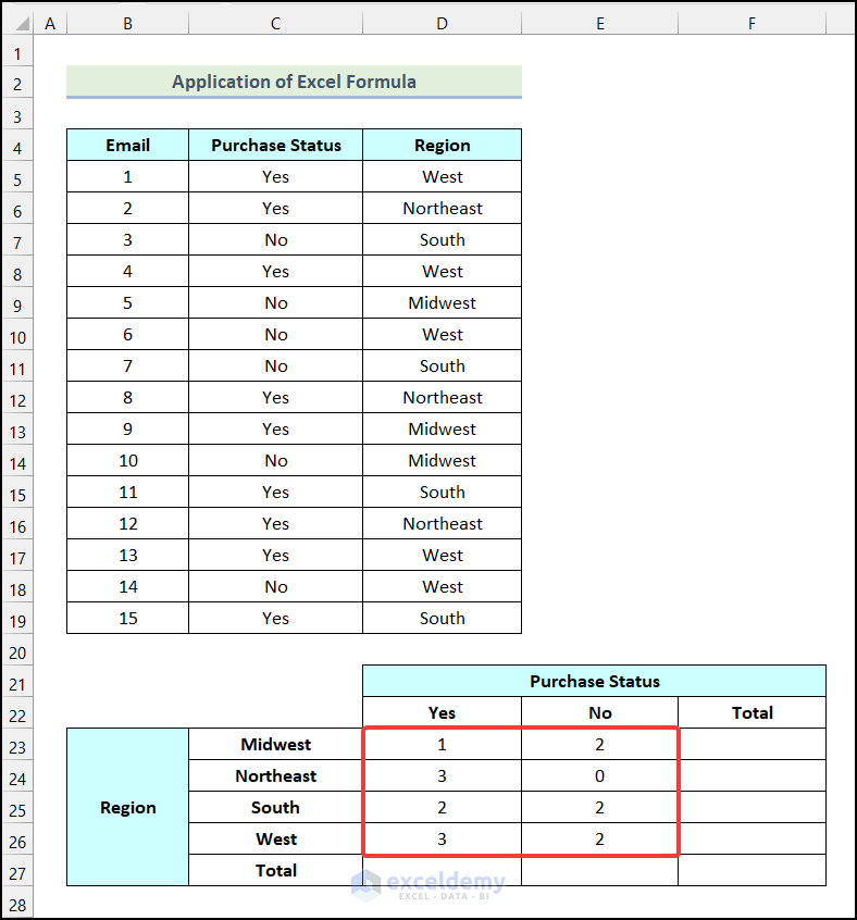
- Drag the Fill Handle to cell E23 to get the following outputs.
- Select cells D23 and E23, then drag the Fill Handle to cell E26.
You will get the count of both the customers who have purchased and didn’t purchase after getting the promotional Email for all Regions, as shown in the image given below.
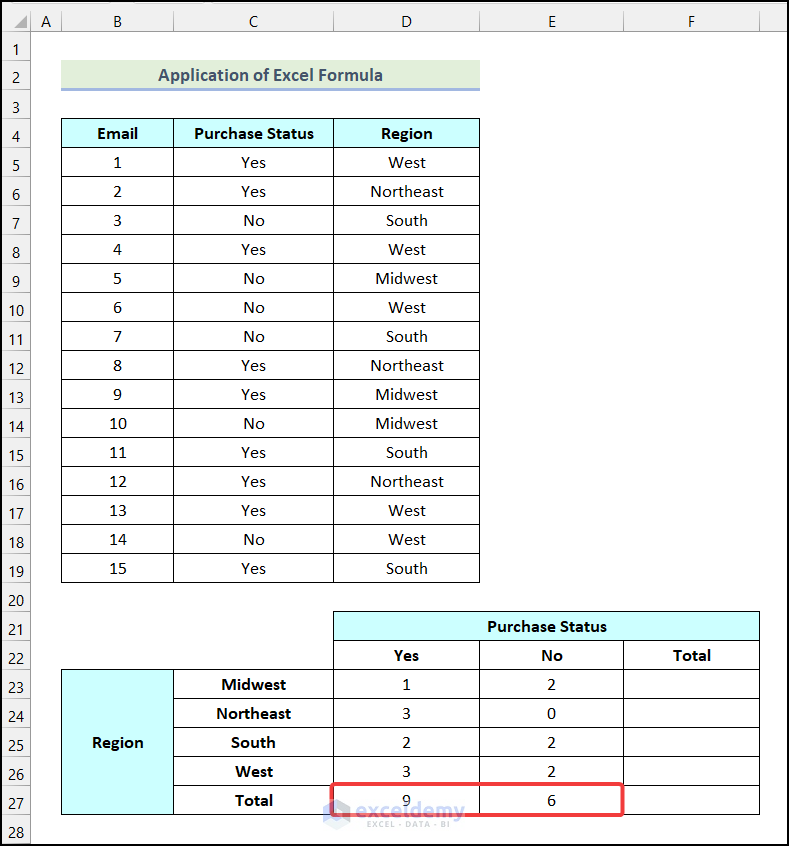
- Enter the formula given below in cell D27.
=SUM(D23:D26)The range of cells D23:D26 indicates the count of customers who have purchased after getting the promotional Email. Then, the SUM function will return the sum of the cells of the selected range.
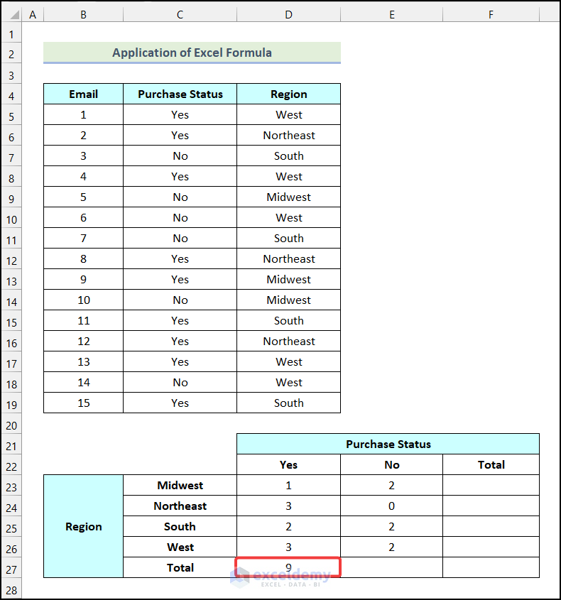
- Hit Enter.
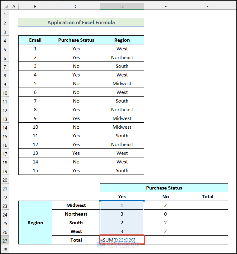
You will get the total number of customers who have purchased after getting the promotional Email in cell D27.
- Drag the Fill Handle to cell E27.
You will get the total number of customers who haven’t purchased after getting the promotional Email in cell E27.
- Use the following formula in cell F23.
=SUM(D23:E23)The range of the cells D23:E23 refers to the count of both the customers who have purchased and didn’t purchase after getting the promotional Email from the Midwest Region.
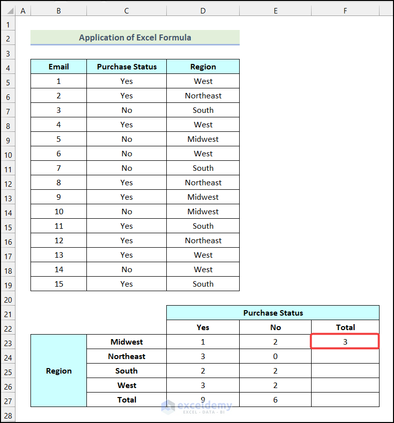
- Hit Enter.
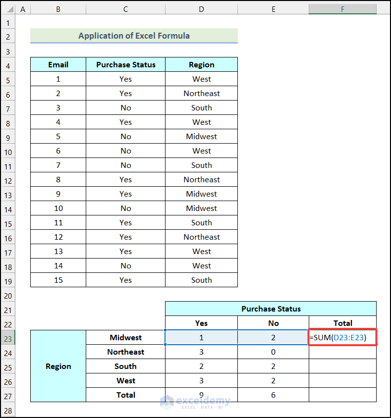
You will get the total number of customers in the Midwest region in cell F23.
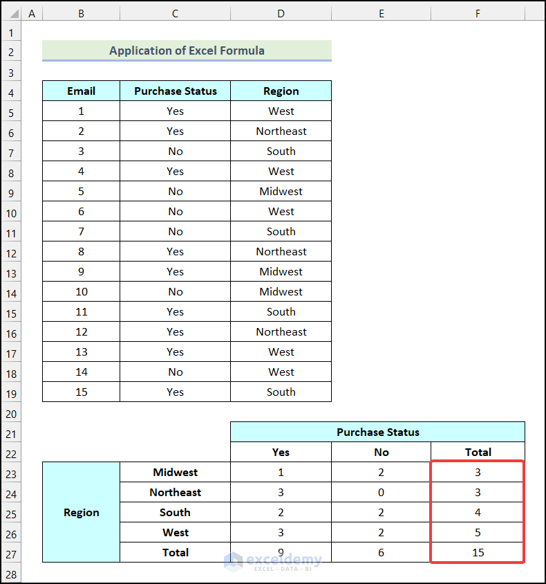
- Drag the Fill Handle to cell F27 to obtain the remaining outputs as demonstrated in the following image.
Read More: How to Make a Relative Frequency Table in Excel
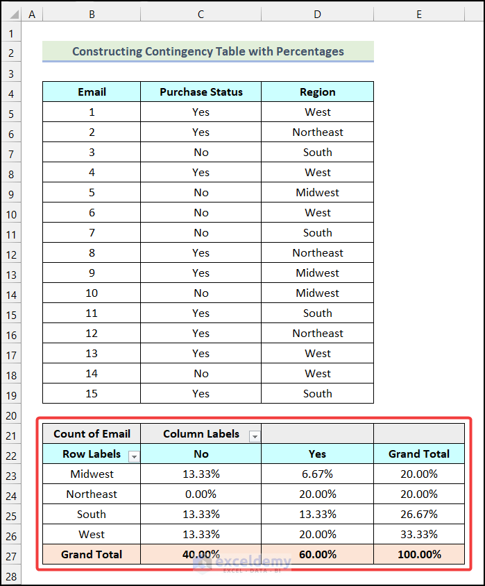
How to Construct a Contingency Table with Percentages in Excel
Steps:
- Follow Method 1 to get the following output.

- Click on any cell of the Pivot Table. We selected cell C23.
The PivotTable Fields dialog box will be available on your worksheet.
- Select the Count of Email as marked in the following image.
- Choose the Value Field Settings option.
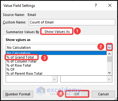
The Value Field Settings dialog box will open on your worksheet.
- Go to the Show Values As tab.
- Click on the drop-down icon as marked in the image below.
- Choose the % of Grand Total option.
- Click OK.
You will get the desired Contingency Table with percentages as demonstrated in the following image.
Read More: How to Make a Categorical Frequency Table in Excel
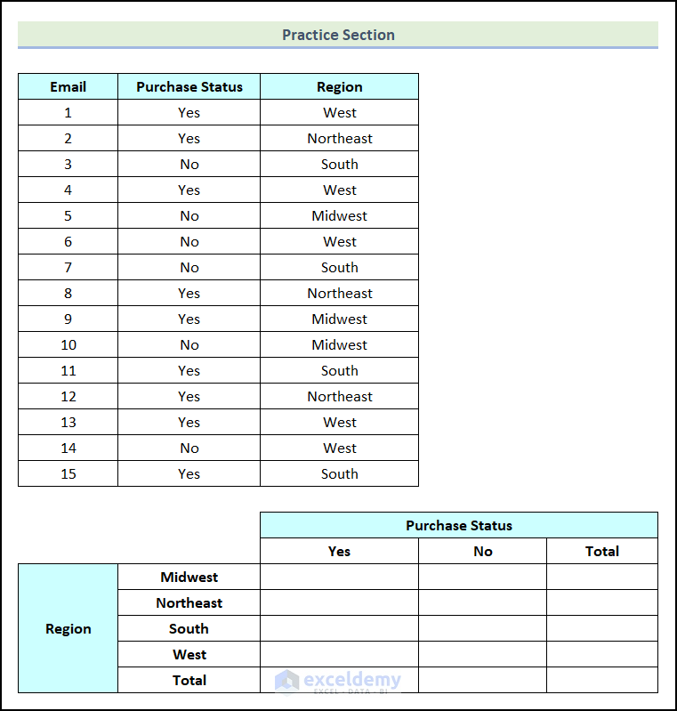
Practice Section
In the Excel Workbook, we have provided a Practice Section on the right side of the worksheet.
Download the Practice Workbook
Related Articles
<< Go Back to Frequency Distribution in Excel | Excel for Statistics | Learn Excel
Get FREE Advanced Excel Exercises with Solutions!
