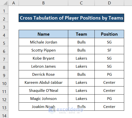
How to Do Cross Tabulation in Excel (3 Suitable Examples)

Method 1 – Cross-Tabulation of Player Positions by Teams

This dataset contains a list of players, their teams, and their positions. We will cross-tabulate how each position is distributed between two teams.

Steps:

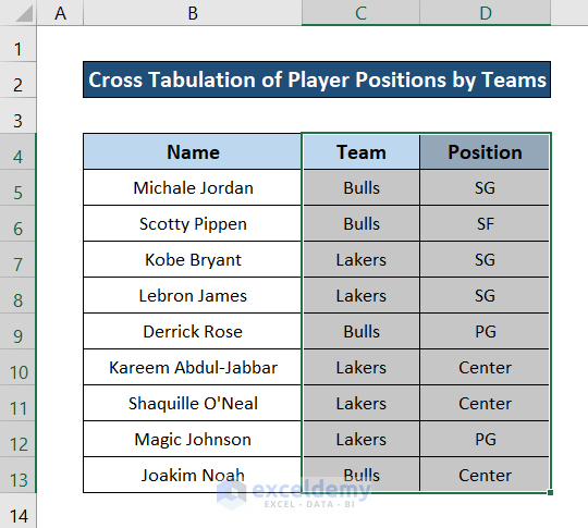
Select the columns you want to base your cross-tabulation.

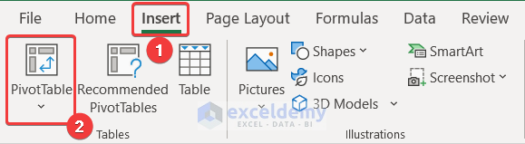
Go to the Insert tab on your ribbon and click PivotTable under the Tables group.

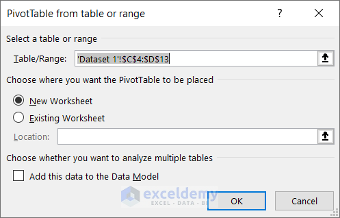
A box will pop up.
Select whether you want your cross tab in the existing worksheet or a new one, and click OK. As shown in the figure, we are selecting a new worksheet for the table.

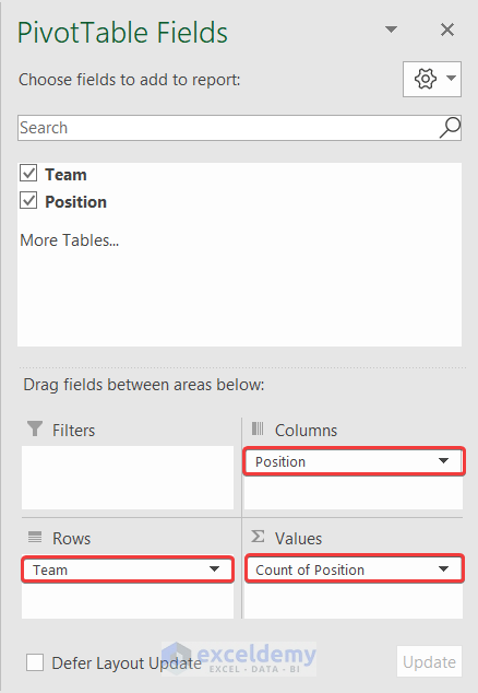
Go to the PivotTable Fields section on the right side of the spreadsheet. You will find the two selected variables- Team and Position.
Click and drag the Team to the Rows.
Do the same for Positions, but this time drag it to both Columns and Values fields.

Excel will automatically organize the pivot table to look something like this.

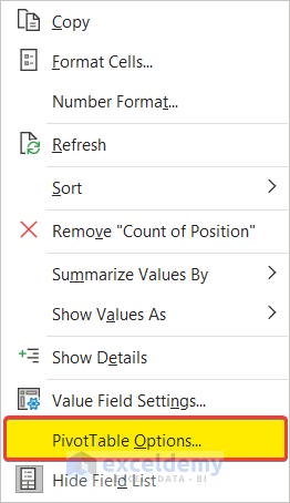
To eliminate the null values, right-click on any table cell and select PivotTable Options from the context menu.

In the PivotTable Options box check the For empty cells show option under Format in the Layout & Format tab and put in the value 0 in it.

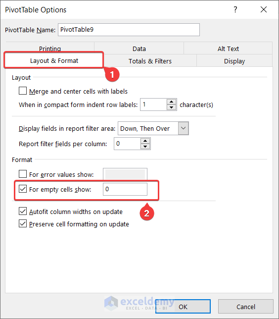
Click on OK.

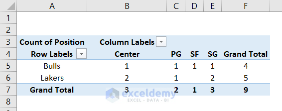
The cross-tabulation is now complete for the dataset. It will look something like this.

Interpretation of the Result

A total of 4 players are from the Bulls, and 5 players are from the Lakers.
The list includes 3 center-positioned players: 2 from the Lakers and 1 from the Bulls.
Both teams have one player who plays as PG.
There is only one player who plays as SF in the dataset, and he plays for the Bulls.
At the same time, there is 1 player plays as SG in the Bulls and two from the Lakers.

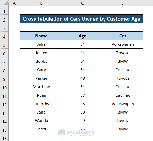
Method 2 – Cross-Tabulation of Cars Owned by Customer Age

Here is a different dataset where there is a possibility of grouping in variables.

Steps:

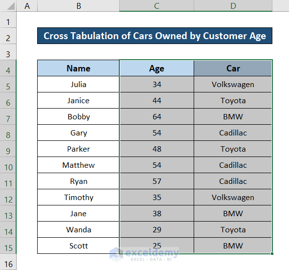
Select the columns for cross-tabulation.

Go to the Insert tab on your ribbon.
Select PivotTables from the Tables group.

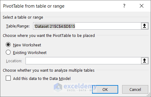
A pivot table box will pop up.
Select where you want your cross tab to be, and click OK.

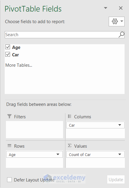
Go to the PivotTable Fields on the right side of the spreadsheet and click and drag Age to the Rows field.
Click and drag Car to both the Columns and Values.

The pivot table will automatically appear at the intended place.

To remove null values, right-click on any cell on the pivot table and select PivotTable options from the context menu.

In the PivotTable Options box, select the Layout & Format.
Check the For empty cells show option and put a 0 in the field.

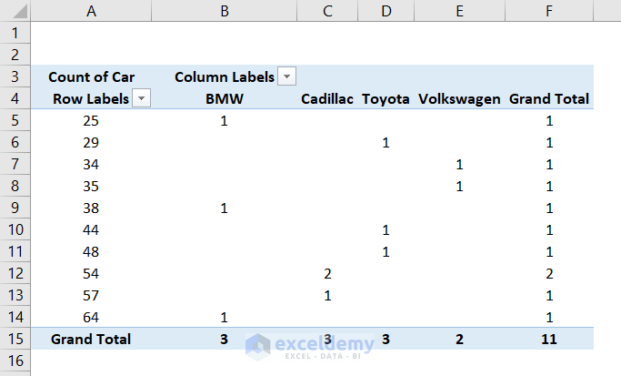
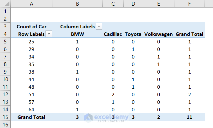
Click OK, and the pivot table will look something like this.

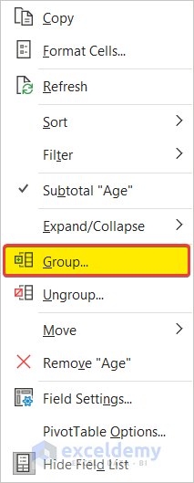
To group the ages. right-click on any row labels and select Group from the context menu.

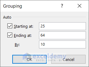
Select the starting, ending, and intervals of the age group you want, and click OK.

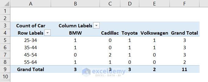
The pivot table will illustrate cross-tabulation, which will look something like this.

Interpretation of the Result

There are 3 people in all 25-34,35-44,45-54 age groups, and 2 people belong to the 55-64 age group.
Of the three people in the 25-34 age category, one owns a BMW, one owns a Toyota, and the other owns a Volkswagen.
One person in the 35-44 age category owns a BMW, one owns a Toyota, and the other has a Volkswagen.
In our next age category of 45-54, two of them own Cadillacs, and one owns a Toyota.
Finally, in our last age group, one person owns a BMW, and another one owns a Cadillac.
It can also be said that Cadillac is popular among older people, and people on the younger side prefer Volkswagen more than their older counterparts. Other cars do not have any age-specific owners.

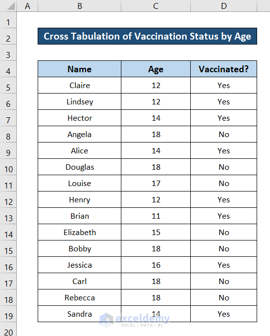
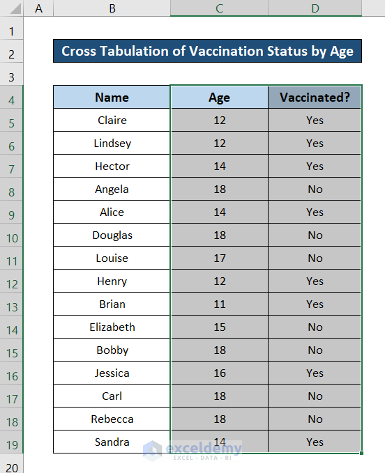
Method 3 – Cross-Tabulation of Vaccination Status by Age

The dataset contains a list of children, their age, and their vaccination status.

Steps:

Select the columns for cross-tabulation.

Go to the Insert tab on your ribbon and select PivotTables from the Tables group.

Select where you want to put the cross tab in and click OK.

Go to the PivotTable Fields on the right side of the spreadsheet. Click and drag Age to the Rows.. Do the same twice for the Vaccinated. variable. It should look something like this, as shown in the figure.

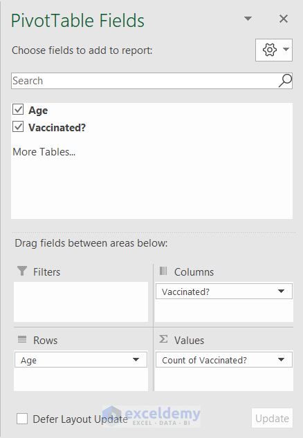
A pivot table will pop up in the spreadsheet that illustrates a cross-tabulation.

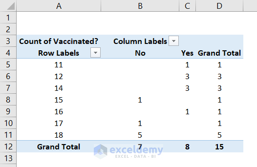
To eliminate the null values, right-click on any of the table’s cells and select PivotTable Options from the context menu.

Select the Layout & Format tab, check For empty cells show option under Format, and put the value 0 in the field.

Click OK, and the cross-tabulation will look something like this.

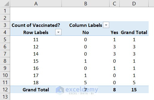
Interpretation of the Result

There is at least one child in every age group from 11 to 18, except 13.
The dataset included 15 children. Seven of these children aren’t vaccinated, while eight are.
The most non-vaccinated children are of age 18, the number of them is 5. None of the 18-year-olds are vaccinated.
Similarly, all 12-year-olds and 14-year-olds are vaccinated. Which is also the dominant age group in terms of vaccination numbers.
The rest of the age groups have only one member. Two are vaccinated, and two aren’t.

Things to Remember

When selecting columns from a dataset for pivot tables, make sure to select all the columns with the headers for the pivot table.
Put the correct variables in the correct fields. You can still work around that, but it involves unnecessary steps for cross-tabulations.
If you want to group the row labels, only click on the cells in the row labels (the first column of the pivot table). Otherwise, the option will not appear on the context menu.

Download the Practice Workbook

Cross Tabulation.xlsx

<< Go Back to Frequency Distribution in Excel | Excel for Statistics | Learn Excel

Get FREE Advanced Excel Exercises with Solutions!