In this tutorial, I am going to share with you 7 practical list of dynamic array formulas in Excel. You can easily apply these functions to perform a wide range of calculations including dynamic array generation inside an Excel worksheet. To achieve this task, we will also see some useful features that might come in handy in many other Excel-related tasks.
How to Create List of Dynamic Array with Formulas in Excel: 7 Easy Examples
1. The UNIQUE Function
Function Objective
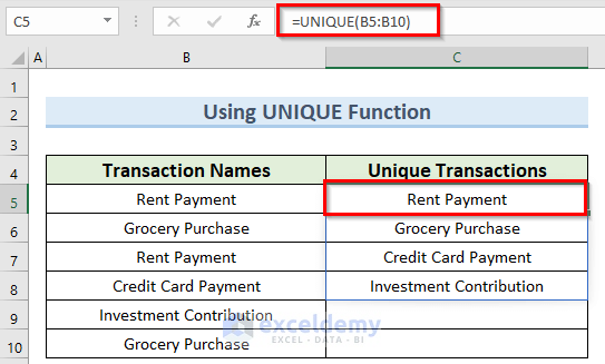
The UNIQUE function in Excel is a function that returns a list of unique values in a range or array. It is often used in combination with other functions, such as the COUNTIF function, to create a list of dynamic array formulas in Excel and to count the number of unique values in a range.
Syntax
UNIQUE(array, [by_col], [exactly_once])
Arguments Explanation
| Argument | Required/Optional | Explanation |
|---|---|---|
| array | Required | Firstly, this is the range or array from which you want to extract unique values. |
| by_col | Optional | When set to TRUE, the function will extract unique values from each column in the range and return them as a vertical array. Otherwise, if set to FALSE (the default), the function will extract unique values from each row in the range and return them as a horizontal array. |
| exactly_once | Optional | When set to TRUE, the function will only return values that appear exactly once in the range. Conversely, if set to FALSE (the default), the function will return all unique values in the range, regardless of how many times they appear. Essentially, setting the “unique” parameter to TRUE will filter out any duplicate values in the range, while setting it to FALSE will include all values, even if they appear multiple times. Also, this can be useful for identifying and removing duplicates in a dataset or for highlighting unique values. |
Return Parameter
The return value of the UNIQUE function is an array of unique values from the specified range or array.
Use of UNIQUE Function
2. The FILTER Function
Function Objective
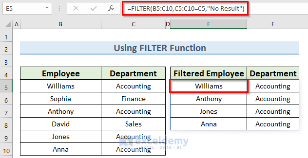
The FILTER function in Excel is a function that allows you to filter a range of data based on specified criteria and return a new set of data that meets those criteria. Additionally, this is the second function in the list of dynamic array formulas in Excel. Furthermore, it is similar to the “Filter” feature in the Data tab, but it allows you to filter data using a formula, rather than manually selecting the criteria.
Syntax
FILTER(range, condition1, [condition2], ...)
Arguments Explanation
| Argument | Required/Optional | Explanation |
|---|---|---|
| range | Required | Firstly, this is the range of cells that you want to filter. |
| condition1, condition2, etc | Required | Similarly, these are the criteria that you want to use to filter the data. Specifically, each condition is a logical test that returns either TRUE or FALSE. As a result, the function will only return cells from the range that meet all of the specified criteria. |
Return Parameter
The FILTER function returns data that meets specific criteria, which can be a single cell, a range of cells, or an array of values, depending on the size and shape of the original data and the criteria being used. Additionally, the type and dimensions of the returned data will vary based on the original data and the criteria being used. Moreover, if the original data is small and the criteria are narrow, the returned data may be a single cell, but if the original data is large and the criteria are broader, the returned data may be a range of cells or an array of values.
Use of FILTER Function
3. The RANDARRAY Function
Function Objective
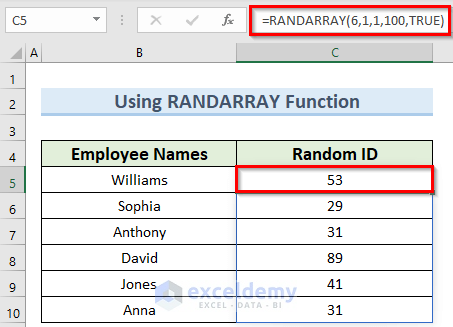
The RANDARRAY function in Excel is a function that generates a random array of numbers between a specified range. Specifically, it can be used to create a set of random numbers for use in statistical analysis or for other purposes.
Syntax
RANDARRAY([rows], [columns], [min], [max])
Arguments Explanation
| Argument | Required/Optional | Explanation |
|---|---|---|
| rows | Optional | Firstly, the number of rows in the array is an optional parameter in the FILTER function. If it is not specified, the default value is 1. In other words, if you do not specify the number of rows in the array, the function will assume that there is only 1 row. Also, this parameter can be useful for controlling the size and shape of the returned data, particularly if you are using the FILTER function to return an array of values. By specifying the number of rows, you can ensure that the returned data is the size and shape that you need for your specific use case. |
| columns | Optional | Similarly, the number of columns in the array is also an optional parameter in the FILTER function. As long as it is not specified, the default value is 1. |
| min | Optional | The minimum value for the random numbers. When not specified, the default is 0. |
| max | Optional | In the same way, it is the maximum value for the random numbers. Whenever not specified, the default is 1. |
Return Parameter
The return value of the RANDARRAY function is an array of random numbers between the specified range. Besides, the size and shape of the array will depend on the values of the rows and columns arguments.
Use of RANDARRAY Function
4. The SEQUENCE Function
Function Objective
The SEQUENCE function in Excel is a function that generates a sequential list of numbers, with a specified step size and starting value. Specifically, it can be used to create a series of numbers for use in statistical analysis or for other purposes.
Syntax
SEQUENCE(rows, [columns], [start], [step])
Arguments Explanation
| Argument | Required/Optional | Explanation |
|---|---|---|
| rows | Required | Firstly, it is the number of rows in the array. |
| columns | Optional | The number of columns in the array. When not specified, the default is 1. |
| start | Optional | The starting value for the sequence. Whenever not specified, the default is 1. |
| step | Optional | The step size for the sequence. In the event that is not specified, the default is 1. |
Return Parameter
The return value of the SEQUENCE function is an array of numbers that form a sequential series, starting at the specified start value and increasing by the specified step value. In addition, the size and shape of the array will depend on the values of the rows and columns arguments.
Use of SEQUENCE Function

5. The SORT Function
Function Objective
The SORT function in Excel is a function that allows you to sort a range of data based on specified criteria. Additionally, it is similar to the Sort feature in the Data tab, but it also allows you to sort data using a formula, rather than manually selecting the criteria.
Syntax
SORT(array, [sort_index], [sort_order], [by_col])
Arguments Explanation
| Argument | Required/Optional | Explanation |
|---|---|---|
| array | Required | This is the range of cells that you want to sort. |
| sort_index | Optional | This is the index of the column or row that you want to sort the data by. As long as not specified, the function will sort the data by the first column or row. |
| sort_order | Optional | This is the order in which you want to sort the data. Now, if this is set to 1 (ascending), the function will sort the data from lowest to highest. In the case that is set to -1 (descending), the function will sort the data from highest to lowest. Also, when not specified, the default is 1 (ascending). |
| by_col | Optional | If and when set to TRUE, the function will sort the data by column. Otherwise if set to FALSE (the default), the function will sort the data by row. |
Return Parameter
The return value of the SORT function is a new set of data that has been sorted according to the specified criteria. The returned data will have the same size and shape as the original data.
Use of SORT Function

6. The SORTBY Function
Function Objective
The SORTBY function in Excel is a function that allows you to sort a range of data based on the values in another range or array. It is similar to the “Sort” feature in the Data tab, but it allows you to sort data using a formula, rather than manually selecting the criteria.
Syntax
SORTBY(array, by_array, [sort_order], [by_col])
Arguments Explanation
| Argument | Required/Optional | Explanation |
|---|---|---|
| array | Required | This is the range of cells that you want to sort. |
| by_array | Required | This is the range or array of values that you want to use to sort the data. Specifically, it must have the same size and shape as the array argument. |
| sort_order | Optional | This is the order in which you want to sort the data. If set to 1 (ascending), the function will sort the data from lowest to highest. Else when set to -1 (descending), the function will sort the data from highest to lowest. Whenever not specified, the default is 1 (ascending). |
| by_col | Optional | Provided that it is set to TRUE, the function will sort the data by column. Else when set to FALSE (the default), the function will sort the data by row. |
Return Parameter
The return value of the SORTBY function is a new set of data that has been sorted according to the values in the by_array argument. Additionally, the returned data will have the same size and shape as the original data.
Use of SORTBY Function

7. The XLOOKUP Function
Function Objective
The XLOOKUP function in Excel is a function that searches for a value in a range or array and returns a corresponding value from a specified column or row. Additionally, it is similar to the VLOOKUP function, but it has additional features and options that make it more flexible and powerful.
Syntax
XLOOKUP(lookup_value, lookup_array, return_array, [match_mode], [search_mode])
Arguments Explanation
| Argument | Required/Optional | Explanation |
|---|---|---|
| lookup_value | Required | This is the value that you want to search for in the lookup_array. |
| lookup_array | Required | This is the range or array of cells that you want to search for the lookup_value. |
| return_array | Optional | Similarly, this is the range or array of cells that contain the values that you want to return. It must have the same size and shape as the lookup_array. |
| match_mode | Optional | This is a number that specifies how the function should match the lookup_value to the values in the lookup_array. When set to 0 (the default), the function will use an exact match. Else whenever set to -1, the function will use the nearest smaller value. In the case that it is set to 1, the function will use the nearest larger value. |
| search_mode | Optional | This is a number that specifies how the function should search the lookup_array for the lookup_value. When set to 1 (the default), the function will search the array in ascending order. Else whenever set to -1, the function will search the array in descending order. If and when set to 2, the function will use a binary search algorithm to search the array. |
Return Parameter
The return value of the XLOOKUP function is the value in the return_array that corresponds to the lookup_value in the lookup_array.
Use of XLOOKUP Function

Download Practice Workbook
You can download the practice workbook from here.
Conclusion
I hope that you were able to apply the methods that I showed in this tutorial on the 7 practical lists of dynamic array formulas in Excel. As you can see, there are quite a few ways to use these functions. So wisely choose the function that suits your situation best. If you get stuck in any of the steps, I recommend going through them a few times to clear up any confusion. If you have any queries, please let me know in the comments.
<< Go Back to Array Formula | Excel Formulas | Learn Excel
Get FREE Advanced Excel Exercises with Solutions!
