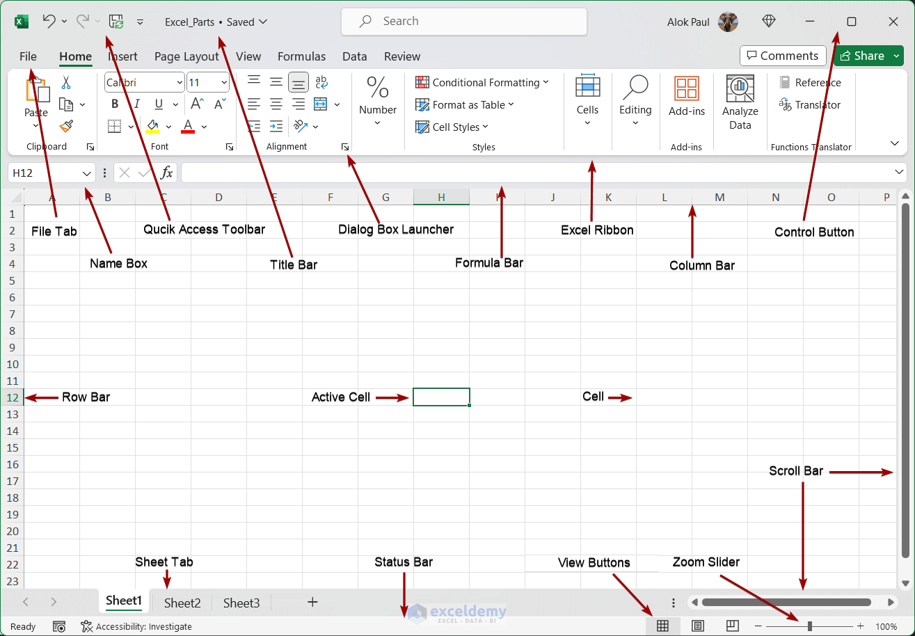
In the following image, you can see the basic parts of an Excel window.
⏷ What Is an Excel Workbook?
⏷ Basic Parts of Excel Window
⏷ Excel Ribbon Structure
⏷ Different Types of Excel Cursors
⏷ Common Excel Dialog Boxes
⏷ Excel Status Bar Options
⏷ Contextual Menus in Excel
⏷ Different Types of Task Panes
What Is an Excel Workbook?
An Excel workbook is an Excel file. It holds one or more worksheets where you can type in, save, and work with data as you like.
Once you launch the Excel application, you will find:
- Options to open a fresh blank workbook
- Recent workbooks you have been working on
- The workbooks that other people have shared with you
- A bunch of ready-made Excel templates
- Excel Account settings
- Feedback section,
- Excel options to customize worksheets and workbooks.
What Are the Basic Parts of the Microsoft Excel Window?
When you open a blank Excel workbook, you will find the following Excel window.
Worksheet: After opening an Excel workbook, we get a window of Excel to perform any required operation that is the worksheet.
Cell: The cell is the shortest part of Excel. Usually, a cell is denoted by the combination of row and column headings. Cell A1 means that the cell is located in the first column and first row. Cell numbers are unique.
Active Cell: When we click on any cell, it becomes the active cell. The address of the active cell is shown in the Name Box at the upper left corner of the sheet.
Row: Row is the horizontal collection of cells and is denoted by a number. On the left side of the sheet, you can see the row bar that indicates all rows. Excel has 1,048,576 rows in total.
Column: The column is the vertical collection of cells and is denoted by alphabetic characters. You will have a bar on the upper side of the worksheet consisting of alphabetic characters starting from A, that is the column bar. Each character of this bar indicates individual columns. Excel has 16,384 columns in total.
Title Bar: The Title bar is the horizontal bar that contains the name of the Excel file and is located at the top of the workbook.
Quick Access Toolbar: The Quick Access Toolbar or QAT is a customized toolbar, located at the left-upper side of the workbook. We gather all the frequently used commands here so that there is no need to search for them.
Control Buttons: Control buttons are located at the upper-right side of the workbook and are used for control purposes like minimizing, maximizing, and closing.
Ribbon: The Ribbon is the key interface in Excel that organizes and contains various commands. It is divided into tabs, each housing groups of related commands. It was first introduced in Excel 2007 and is available in all the latest versions including Excel 365.
Formula Bar: Formula bar is located below the ribbon. We can insert, modify, and delete any value or formula in Excel from this bar. We can also see the formula of any cell in this bar.
Name Box: The Name Box is on the left side of the Formula Bar. We can see the address cell or name of a range from this box. We can also go to the desired cell or select the range by inserting the cell reference or name in this box.
Scroll Bar: The scroll bar is used to navigate the Excel worksheet in 4 directions. There are two scroll bars: the horizontal scroll bar for left and right, and the vertical scroll bar for up and down directions.
Sheet Tab: The sheet tab contains the names of all available sheets on the workbook. We can also create new sheets from there. It is also called the leaf bar. It is located at the bottom left corner of a workbook above the Status Bar.
Status Bar: The status bar is a horizontal bar located at the bottom of the workbook. It indicates the current status of the selected cell and other mathematical calculations like sum, average, count, etc.
Zoom Slider: It refers to the zoom adjustment of Excel workbooks that ranges from 10% to 400%. It is located at the bottom-right corner of the Excel workbook.
View Buttons: This button refers to different ways to present the workbook in Excel. There are three modes: Normal, Page Layout, and Page Break Preview.
How Is the Excel Ribbon Structured?
The Excel ribbon has the following basic components: Tabs, Command Groups, Command Buttons, and Dialog Box Launcher.
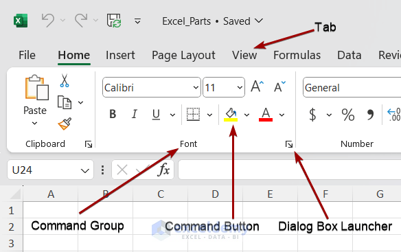
Tab: A tab is an entity that organizes a similar group of commands in Excel. Each tab stands for a specific purpose. Like, the Insert tab is used to insert tables, illustrations, charts, maps, sparklines, etc. in the dataset.
Command Groups under Each Tab: Under each tab, there are multiple command groups to do specific tasks. Example: The Font group under the Home tab is dedicated to font size, color, style, and other font-related tasks.
Command Buttons under Each Group: These are different buttons under each command group. Each command button performs a specific task. Example: the Font Color button sets the color of the font.
Dialog Box Launcher: The dialog box launcher is a small arrow symbol located at the bottom-right side of any command group. Some command groups contain more commands than shown in the Ribbon. The dialog launcher (also called an anchor arrow) shows the other commands related to each group in a pop-up window.
What Are the Different Types of Cursors Used in Excel?
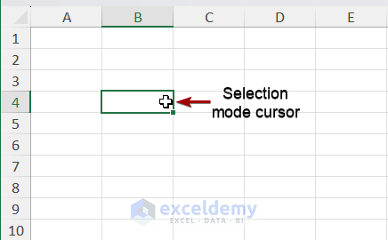
Type 1 – Selection Mode Cursor
When you hover the cursor over a cell or select a cell, the cursor looks like this.
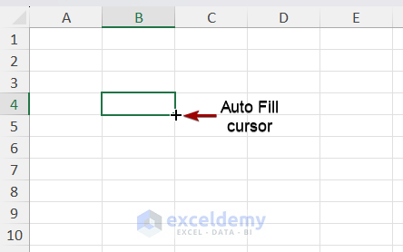
Type 2 – AutoFill Cursor or the Fill Handle
It is a small plus sign when hovering over the right-bottom corner of a cell. Clicking and dragging or double-clicking on the cursor will copy the formula or values inside to subsequent cells.
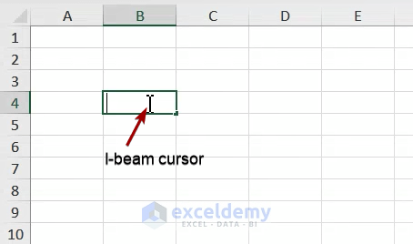
Type 3 – I-Beam Cursor
The I-beam cursor is displayed when entering values into cells directly.
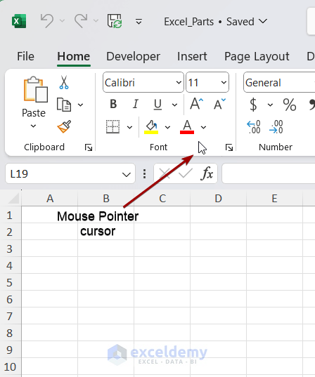
Type 4 – Mouse Pointer Cursor
The mouse pointer shows up when hovering over anything that’s not a cell or text box.
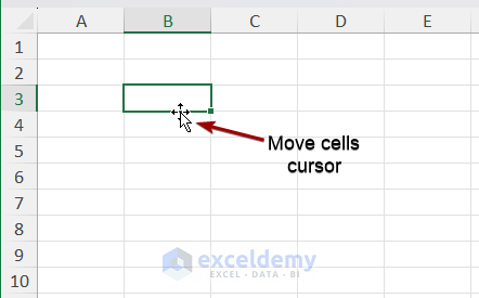
Type 5 – Move Cells Cursor
It looks like a four-directional arrow sign and appears when placing the cursor at the edge of the selection range. Dragging the cursor to another location will move the selected data.
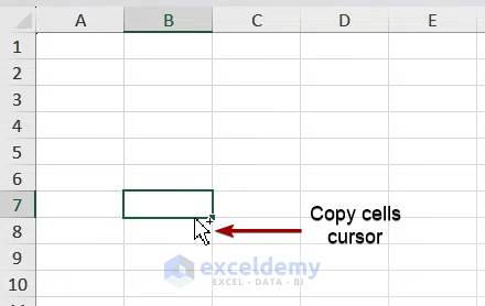
Type 6 – Copy Cells Cursor
Place the cursor on the edge of the selection area, then press and hold the Ctrl button. You will see a small plus icon with the mouse pointer, which is Copy Cells cursor. Using this cursor, you can copy, move, and do other activities.
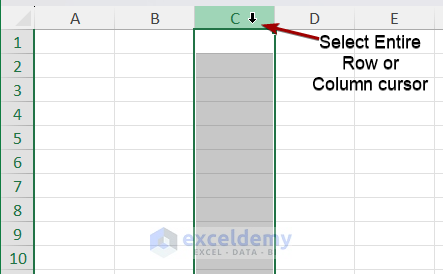
Type 7 – Cursor to Select Row/Column
It appears when you hover over the column or row bar and turns the cursor into a down or right arrow. It’s used to select the entire column or row.
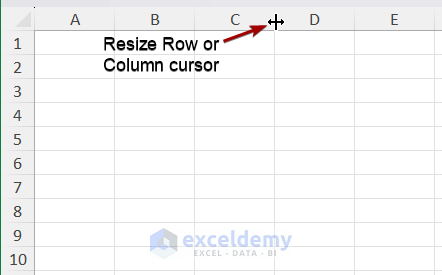
Type 8 – Cursor to Resize Column/Row
When the cursor is placed at the border of two columns or rows, it will turn into a two-directional arrow. It can resize the width or height of a column or row, respectively.
What Are the Common Excel Dialog Boxes?
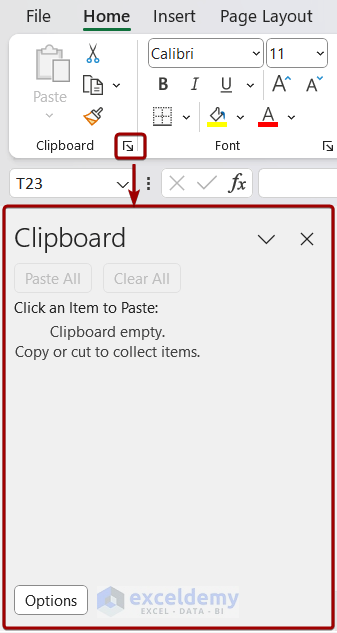
Type 1 – Clipboard Dialog Box
We get this dialog box from the Clipboard group of the Home tab. Our copied data is shown in this dialog box.
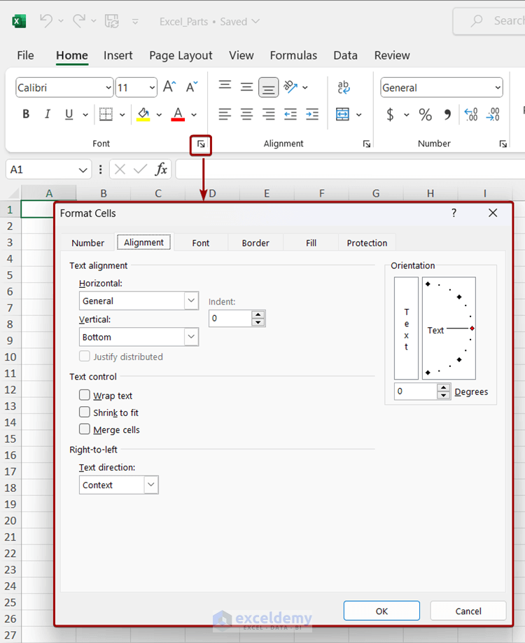
Type 2 – Format Cells Dialog Box
Opened from the Font, Number, or Alignment group of the Home tab. Used to customize the data format like category, size, color, style, alignment, add a border, fill color, etc.
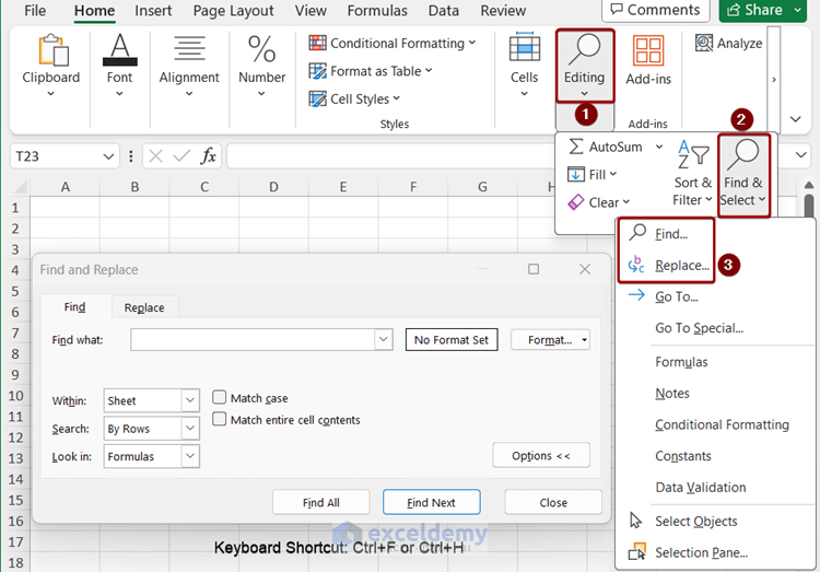
Type 3 – Find and Replace Dialog Box
Pressing Ctrl + F or H will get this dialog box. Also opened via Find & Select > Find or Replace. From the Find tab, you can search for any data, and from the Replace tab you can replace the existing data with new ones.
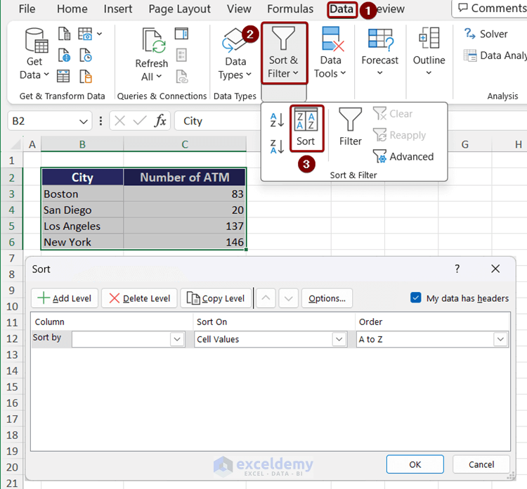
Type 4 – Sort Dialog Box
Go to Find & Select and choose Custom Sort to get this dialog box. You can sort data in multi-level and multiple categories from this dialog box.
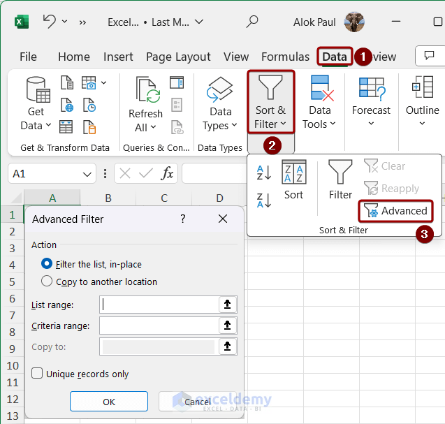
Type 5 – Advanced Filter Dialog Box
Go to Sort & Filter and select Advanced to open it. You can select both the data and criteria range and apply the advanced filter from this box.
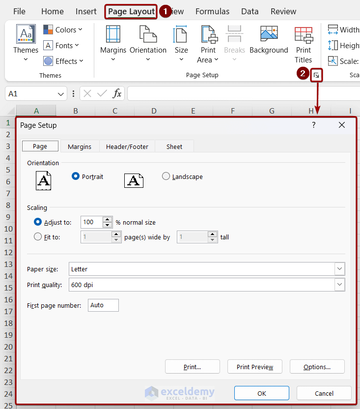
Type 6 – Page Setup Dialog Box
Opened via the Page Layout tab. Click on the dialog box launcher of groups Page Setup, Scale to Fit, or Sheet Options. You can use it to customize page orientation, scaling, paper size, margin, header, footer, print area, page order in printing, etc.
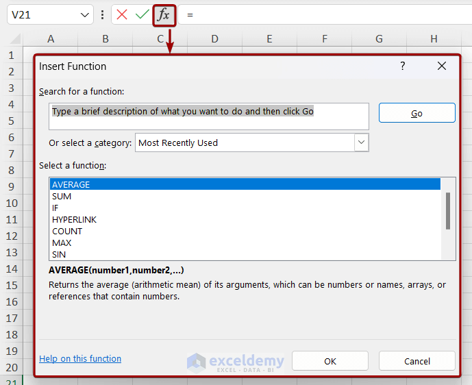
Type 7 – Insert Function Dialog Box
You can open the Insert Function dialog box by clicking on the fx sign next to the Formula Bar. You will get the list of Excel functions based on different categories to insert into the formula bar.
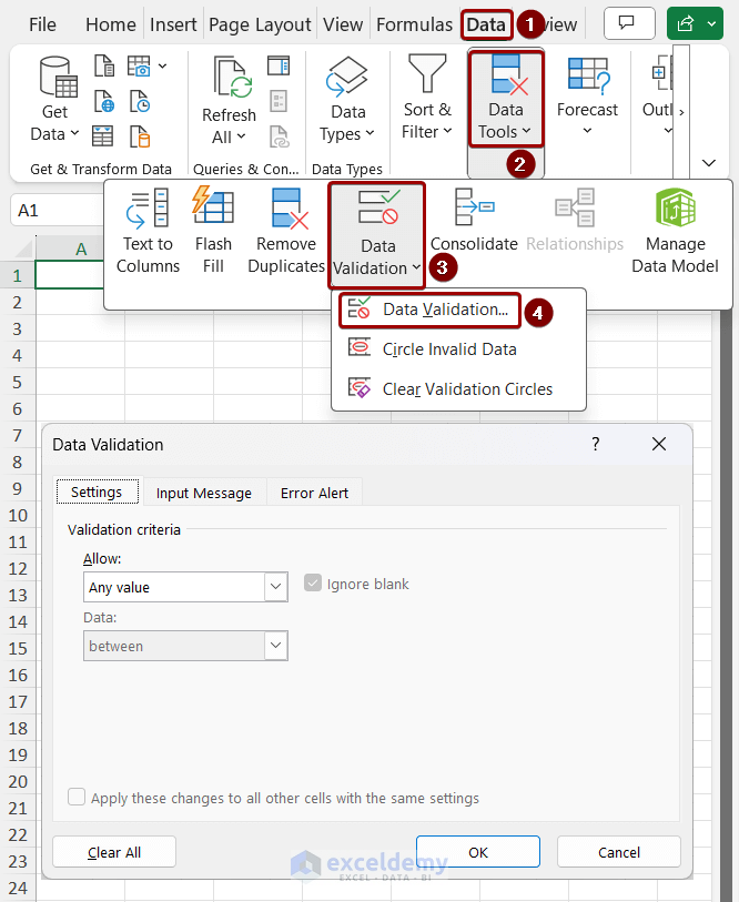
Type 8 – Data Validation Dialog Box
Go to Data and select Data Validation to get this dialog box. It allows you to control the entry of data in a cell.
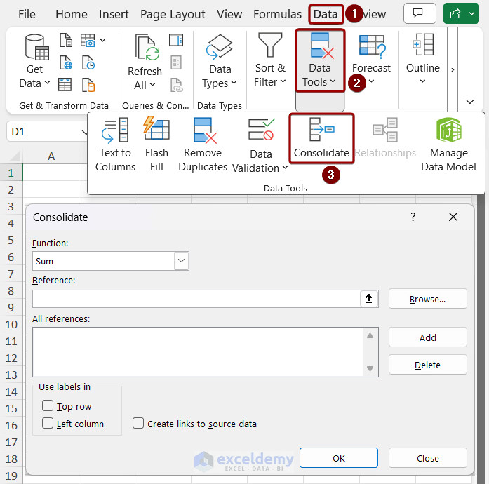
Type 9 – Consolidate Dialog Box
You will get this dialog box by going to Data and selecting Consolidate. It summarizes information from multiple worksheets into a master worksheet.
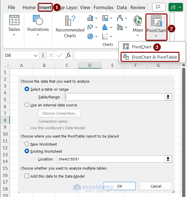
Type 10 – PivotTable and PivotChart Wizard
Go to Insert and select the PivotChart drop-down, then choose PivotChart & PivotTable to get this dialog box. Select a table or range as source data and another location to place the pivot table and chart in the workbook.
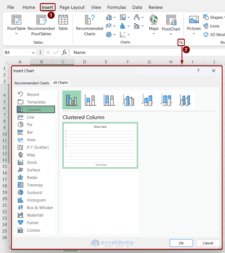
Type 11 – Insert Chart Dialog Box
Click on the dialog box launcher of the Charts group of the Insert tab. You can select the desired chart from the recommended options or a list of all charts.
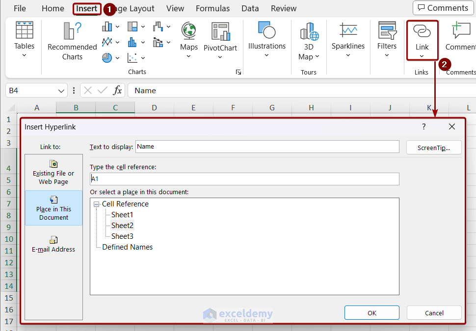
Type 12 – Hyperlink Dialog Box
To get this box, click on the Link command in the Insert tab. You can link any file (Image, document, etc.), web page, sheets of the existing workbook, and email address.
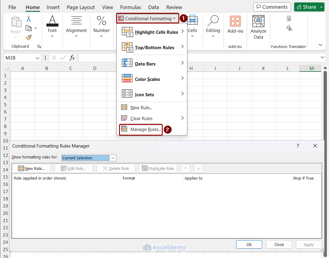
Type 13 – Conditional Formatting Dialog Box
In Home, go to Conditional Formatting and select Manage Rules to get this dialog box. You can create, edit, delete, and duplicate conditional formatting rules from this box.
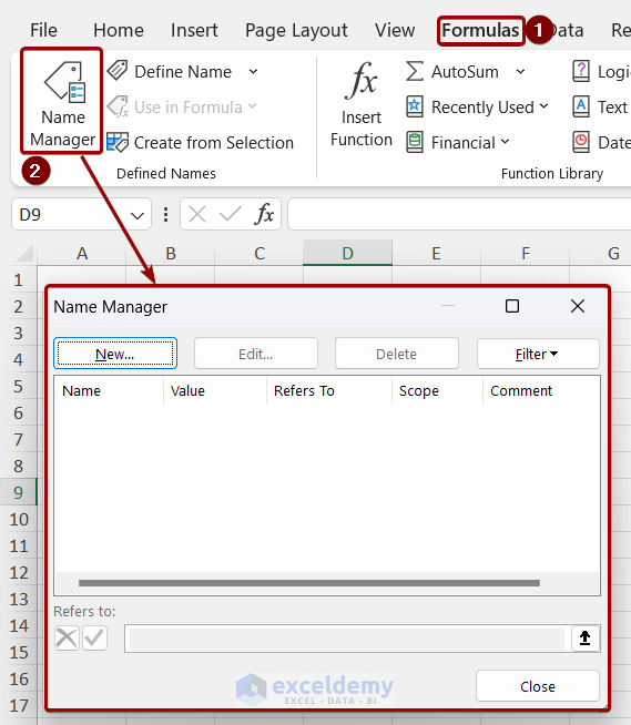
Type 14 – Name Manager Dialog Box
Go to Formulas and select Name Manager. It can be used to create, edit, and delete names for ranges. You can also modify the reference of shown names from here.
What Are Excel Status Bar Options?
The status bar is the horizontal bar at the bottom of the workbook. By default, this bar shows a real-time status of the workbook: Cell Mode, Macro recording, Accessibility, mathematical calculations, View buttons, and Zoom Slider.
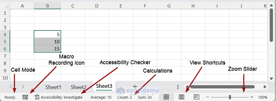
- The Cell Mode indicates different modes of cells like ready, edit, enter, and point.
- When the Macro Recording icon is active, Excel records all the actions and converts them into VBA so that we can use it later.
- The Accessibility Checker checks is a tool that checks the usability of each worksheet and suggests how to fix them.
- The mathematical calculations section shows the average, count, sum, and other calculations by selecting the desired cells only.
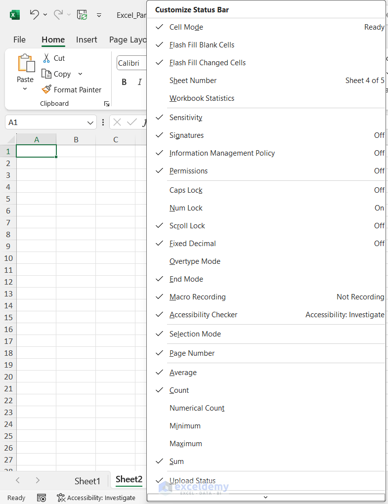
Here’s how you can customize it:
- Right-click over the Status Bar.
- The Customize Status Bar menu will appear.
- Check the desired option from the menu to appear in the Status Bar.
You can hide or unhide the status bar easily by using the keyboard shortcut Ctrl + Shift + F1.
What Are the Contextual Menus in Excel?
The Context Menu appears by right-clicking on any object like a cell, chart, shape, or command. Here is a cell’s context menu.
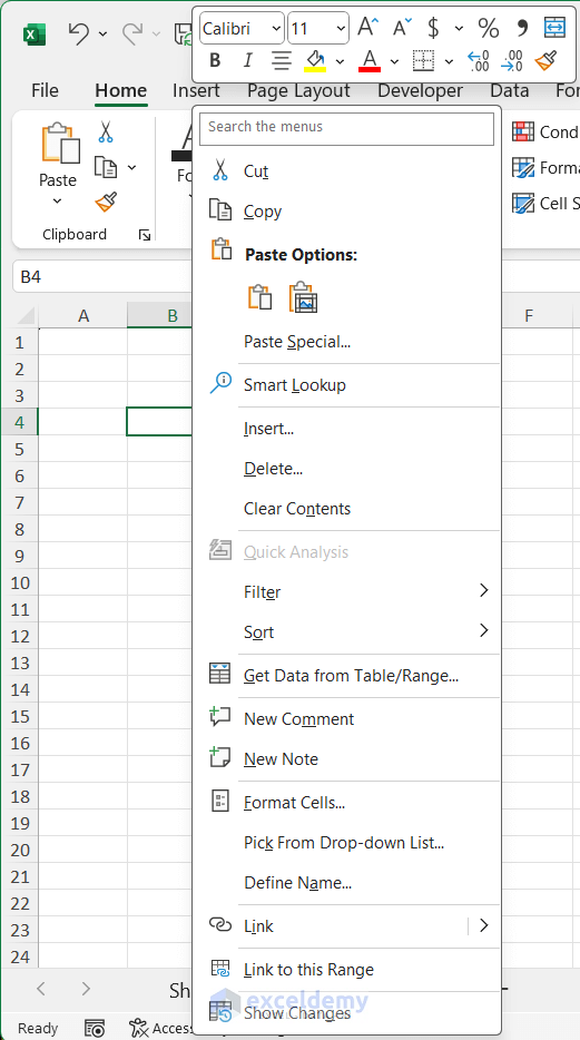
Type 1 – Context Menu That Appears After Right-Clicking on Cells
Options in this context menu are related to the data in a cell like: copy, cut, paste, sort, filter data, insert, delete, format cells, etc.
Type 2 – Context Menu of Ribbon
The features of this menu are related to the Quick Access Toolbar and the ribbon.
We get two types of context menus from the ribbon:
- Right-click on the Tab or blank space of the ribbon.
- Right-click after placing the mouse over a ribbon command.
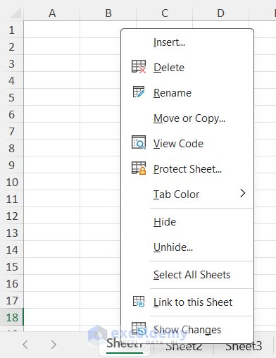
Type 3 – Context Menu of the Sheet Tab
Hover the mouse over any sheet name of the Sheet Tab and get this menu. It consists of options like insert, delete, rename, move, copy sheets, etc.
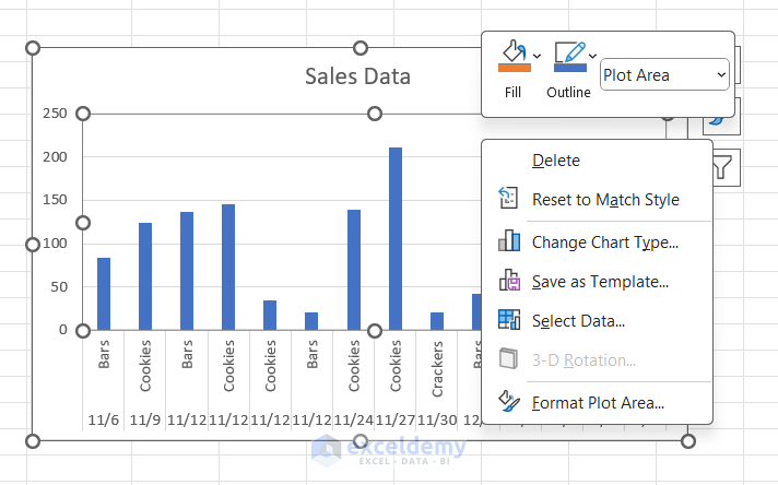
Type 4 – Context Menu of a Chart
It’s used to change the fill color, outline color, chart type, data, etc. of a chart.
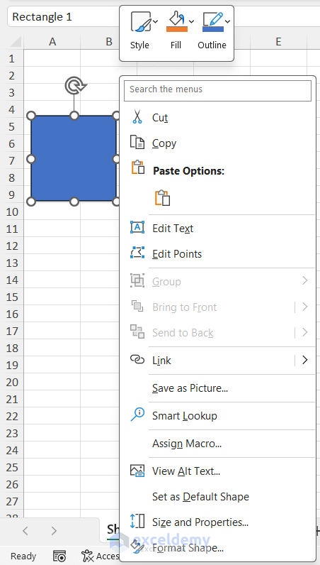
Type 5 – Context Menu of a Shape
You can modify texts, points, links, size, and other properties of shape from this menu.
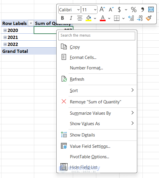
Type 6 – Context Menu of a Pivot Table
You can modify the font style, color, size, and format of data and show different mathematical calculations and other options related to the pivot table from this menu.
What Are Different Types of Task Panes in Excel?
Task Pane is a supporting tool of Excel. Usually, a Task pane is shown in a rectangular box. Each task pane shows different functionality, such as selecting any option, inserting a value, etc.
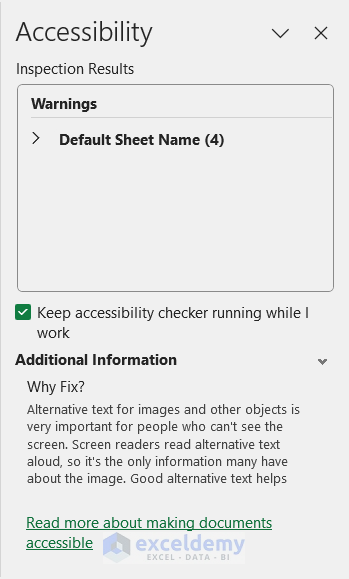
Type 1 – Accessibility Checker
This task pane checks the accessibility of the workbook and suggests how to make the workbook more accessible after fixing disabilities.
Click on the Accessibility Checker icon on the left side of the Status Bar and the task pane will be located on the right side of the workbook.
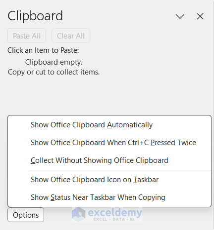
Type 2 – Clipboard
This task pane is accessed from the Clipboard group of the Home tab and appears on the left side of the workbook. It lists the copied data, and we can paste or delete it from the Clipboard.
There is also an Options button at the bottom of the taskbar with other features.
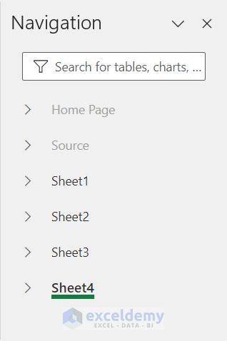
Type 3 – Navigation
Click on the Navigation feature of the View tab to open this task pane. In this pane, you can view all the elements, such as tables, images, charts, PivotTables, and datasets, of each worksheet of the workbook.
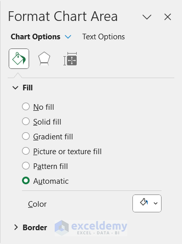
Type 4 – Format Chart Task Pane
We will get this by right-clicking on a chart. This task pane shows all the chart’s properties for customization.
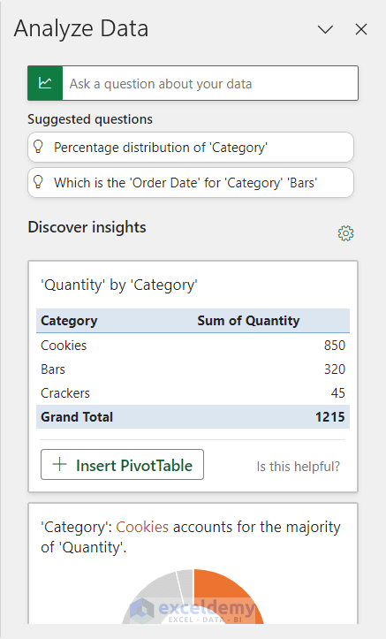
Type 5 – Analyze Data
Select a range of data and click on the Analyze Data feature of the Home tab to get this task pane. You can see different insights of the dataset and can ask any question regarding the dataset. Previously, it was called Ideas.
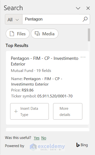
Type 6 – Smart Lookup
Accessed from the Smart Lookup option of the Review tab. This task pane shows definitions, images, web pages, and related information of the selected data after searching.
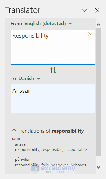
Type 7 – Translator
This task pane shows the translation of the inserted word or sentence. You can access it by clicking on the Translate option under the Review tab.
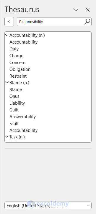
Type 8 – Thesaurus
This task pane shows the synonyms and antonyms of inserted words in Excel. Click on the Thesaurus option of the Proofing group under the Review tab to access it.
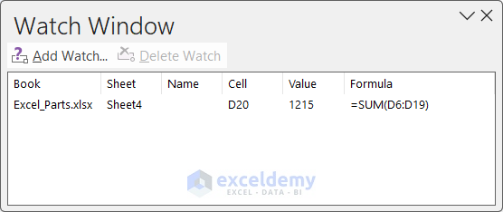
Type 9 – Watch Window
You will be able to see all the details of a cell in this task pane like the workbook name, sheet name, value, formula, etc. of the selected cell. Click on the Watch Window option of the Formulas tab for this pane.
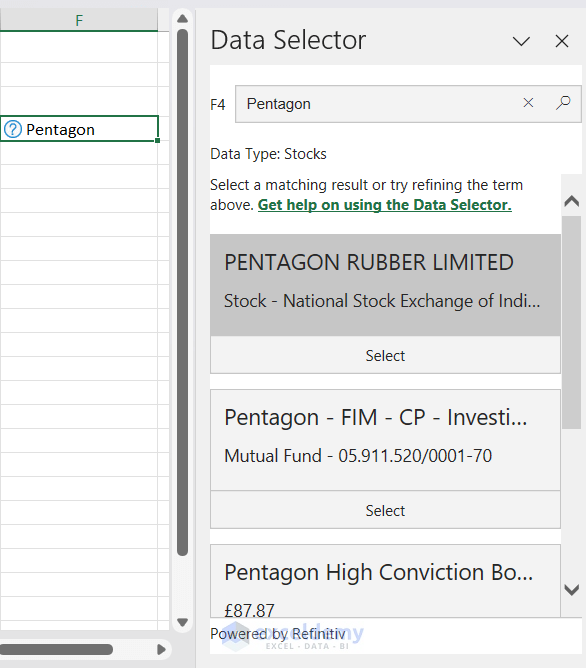
Type 10 – Data Selector
The Data Selector task pane appears when you change the data type of the inserted data from the Data Types group under the Data tab. This task pane shows suggestions based on your data type selection.
Excel Parts: Knowledge Hub
<< Go Back to Learn Excel
Get FREE Advanced Excel Exercises with Solutions!
