How to Create and Use Scroll Bar in Excel (3 Easy Ways)

A scroll bar is a tool for displaying huge data tables from top to bottom or left to right and vice versa.

Here is an overview of an Excel data table with a Scroll Bar.

Download the Practice Workbook

Scroll Bar.xlsm

What Is a Scroll Bar in Excel?

A scroll bar is a slider in Excel that allows you to examine data from left to right or top to bottom.

There are two types of scroll bars in Excel. They are:

Vertical Scroll Bar
Horizontal Scroll Bar

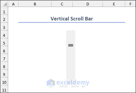
Vertical Scroll Bar: A vertical scroll bar is a tool for viewing data from top to bottom.

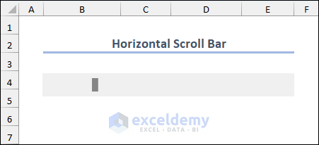
Horizontal Scroll Bar: A horizontal scroll bar is a tool for viewing data from left to right.

How to Create a Scroll Bar in Excel?

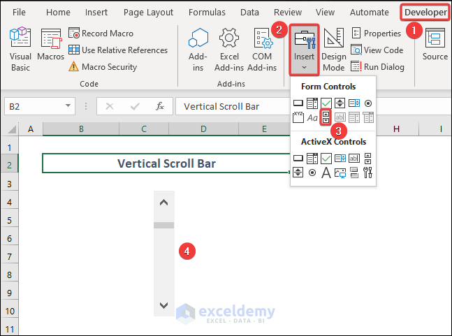
To create a Scroll Bar in Excel, go to Developer, then select Insert and choose Scroll Bar from Form Control.
Draw the Scroll Bar and drag the cursor it to give it the shape of a vertical or horizontal Scroll Bar.

What Are the Ways to Create a Scroll Bar in Excel?

Create a Vertical Scroll Bar in Excel

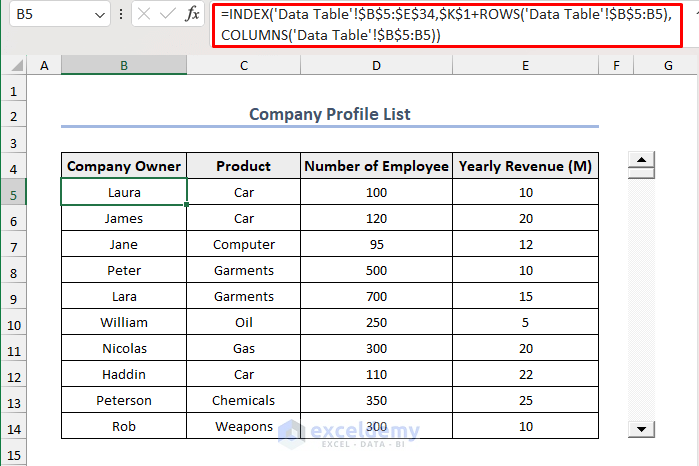
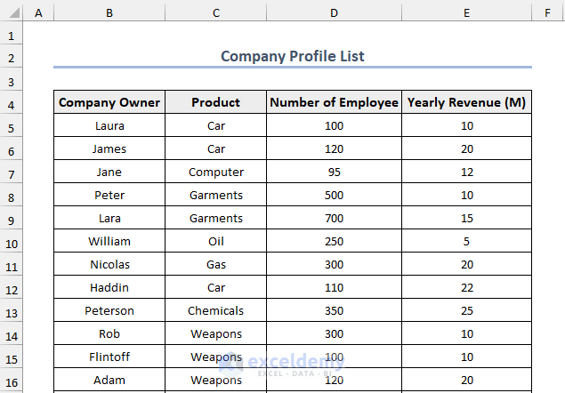
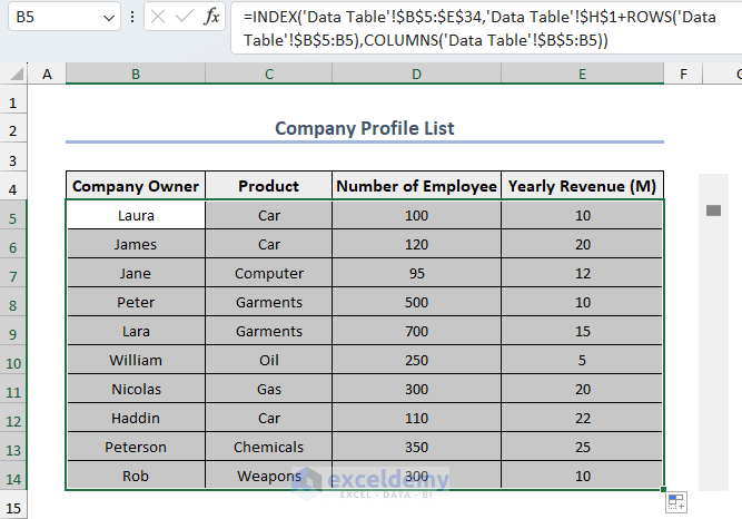
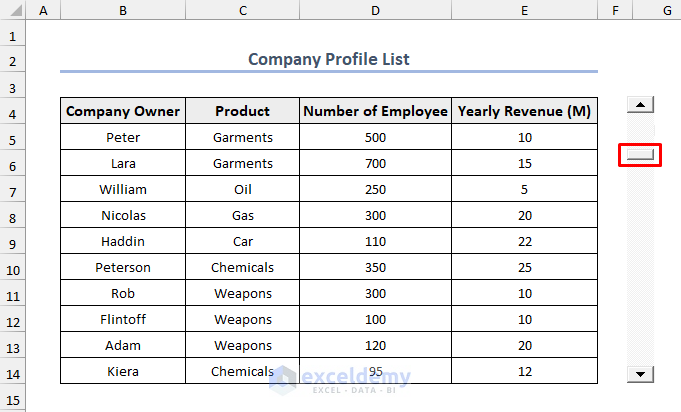
In the following image, you will see a part of a data table that contains 30 rows excluding the column headings. We cannot see all the rows in the Excel sheet because the number of visible rows for an Excel sheet is limited for monitors of different sizes. To show this data table with a Scroll Bar, we’ll create a dataset with the same column headings and create a vertical Scroll Bar.

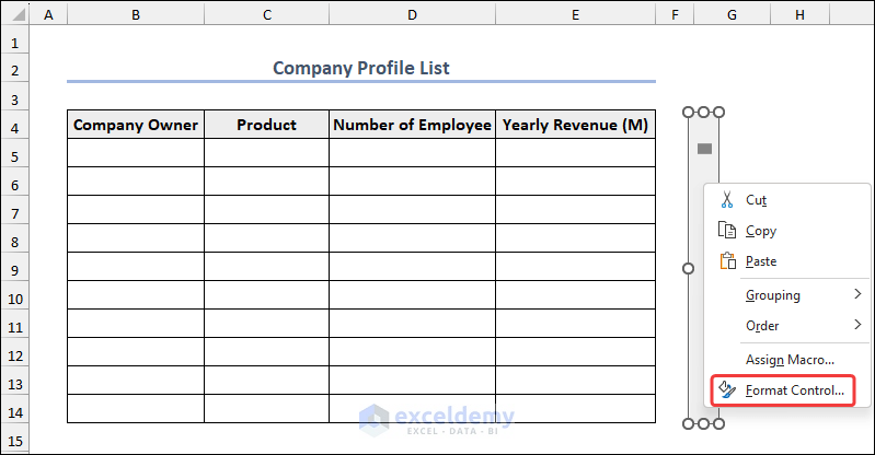
Right-click on the Scroll Bar and select Format Control from the Context Menu.

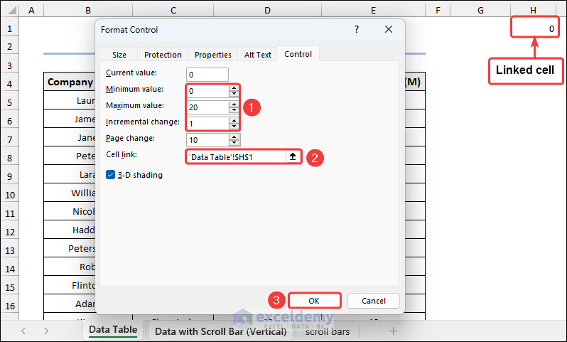
In the Format Control dialog box, insert the parameters. In our case, we have a data table of 30 rows and 10 of them will be displayed by the Scroll Bar. So, we set the Minimum and Maximum Value to 0 and 20.
The Scroll Bar is linked to the H1 cell of the Data Table The value of this cell changes from 0 to 20 while clicking on the down or up arrows of the Scroll Bar.

Click the image to get a detailed view

Use the formula below to change the data with the Scroll Bar.

=INDEX('Data Table'!$B$5:$E$34,'Data Table'!$H$1+ROWS('Data Table'!$B$5:B5),COLUMNS('Data Table'!$B$5:B5))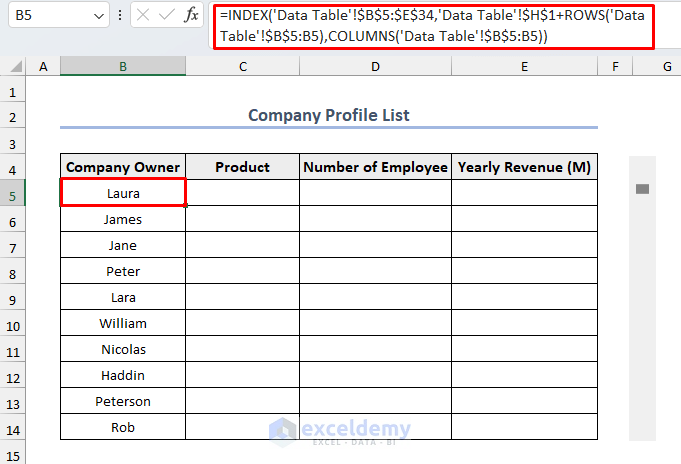

Formula Breakdown

‘Data Table’!$B$5:$E$34: This refers to the range of cells B5 to E34 in the worksheet named Data Table. It represents the array from which we want to retrieve the value.
‘Data Table’!$H$1+ROWS(‘Data Table’!$B$5:B5): This part calculates the row offset for the INDEX function. It takes the value in cell H1 in the Data Table worksheet and adds the number of rows from B5 to the current row (B5 to B5, B5 to B6, B5 to B7, and so on). The value of the H1 cell changes and thus changes the data in the table with each Scroll Bar This creates a dynamic offset as the formula is copied down the column.
- Output: 1
COLUMNS(‘Data Table’!$B$5:B5): This returns the column offset for the INDEX It counts the number of columns from B5 to the current column. Similar to the previous step, this creates a dynamic offset as we copied the formula across the row.
- Output: 1
INDEX(‘Data Table’!$B$5:$E$34,1,1): Here, we used the INDEX function to retrieve the value at the specified row and column offsets within the given array. The row offset is determined by the value in cell H1 and the number of rows from B5 to the current row. The column offset is determined by the number of columns from B5 to the current column.
- Output: Laura

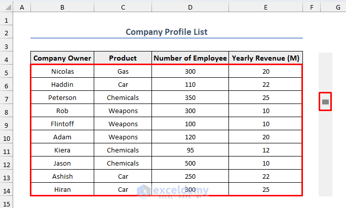
Copy the formula to other columns with the Fill Handle to get all the elements of the corresponding table.

Scroll down and you will see the lower rows of the table in the Data Table sheet.

Create a Horizontal Scroll Bar in Excel

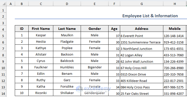
When your data table contains a lot of columns, using the horizontal Scroll Bar is paramount. Here is a part of the data table that contains 9 columns. We cannot display all the columns on one page of an Excel sheet.

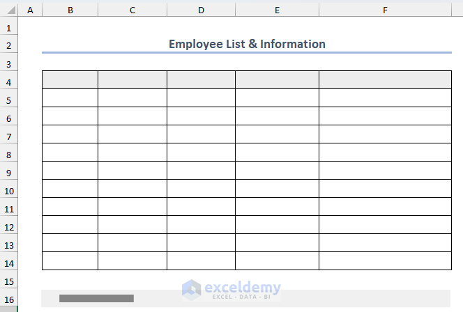
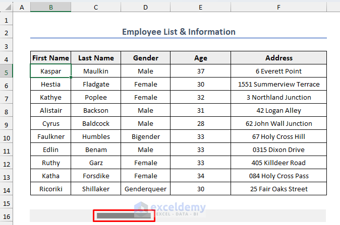
We made a blank data table with 5 columns. The above data will be displayed with a horizontal Scroll Bar in this table.
We created a horizontal Scroll Bar and formatted its parameters. See the section on creating a vertical scroll bar above for details.

Use the formula below to extract the data in the new sheet. Apply the Fill Handle to copy the formula all over the data table which populates the blank cells with corresponding data.

=INDEX('Data Table (for Horizontal)'!$B$4:$J$14,ROWS($B$5:B6),'Data Table (for Horizontal)'!$L$3+COLUMNS($B$5:B6))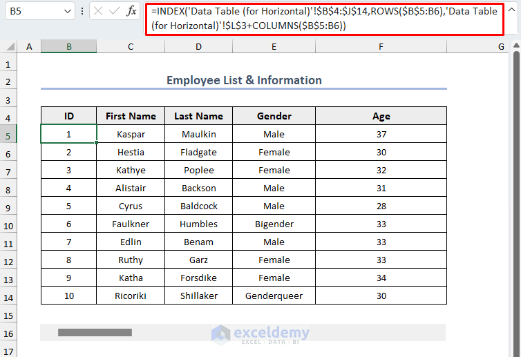

Click on the right side of the Scroll Bar to see the adjacent columns.

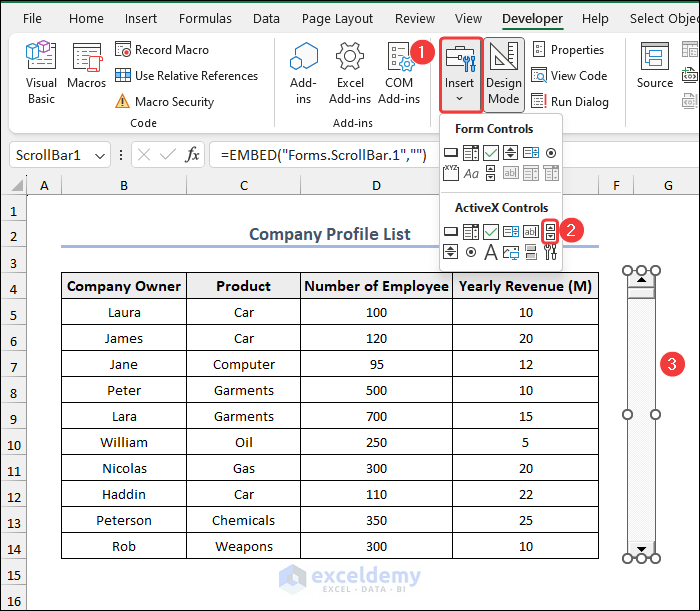
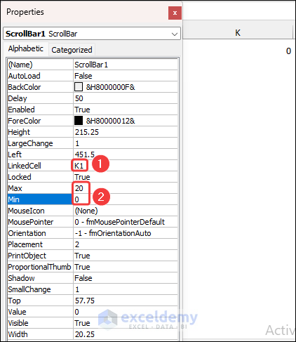
Create an ActiveX Scroll Bar in Excel

Create a Scroll Bar from the ActiveX Controls group. Select Developer, then Insert, and finally, ActiveX Scroll Bar.
Draw the Scroll Bar to a suitable size. Drag and resize if needed.

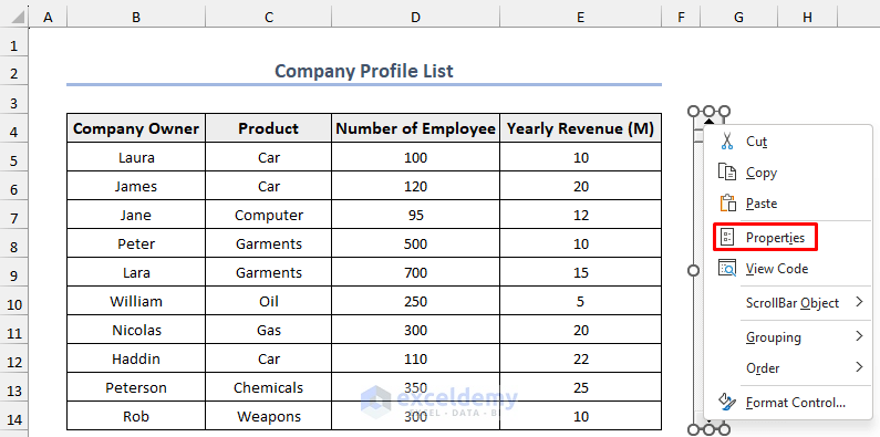
Open the Properties window for the Scroll Bar from the Context Menu.

Set up Linked Cell, Max, and Min values like in the Vertical Scroll Bar section.

Copy the formula below for the Scroll Bar.

=INDEX('Data Table'!$B$5:$E$34,$K$1+ROWS('Data Table'!$B$5:B5),COLUMNS('Data Table'!$B$5:B5))

This is the same formula we used for the Vertical Scroll Bar. The only difference is the Linked Cell reference used in the formula.

You can scroll down the ActiveX Scroll Bar to see the unseen data of the data table.

How to Hide the Default Scroll Bar in Excel?

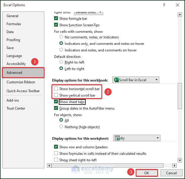
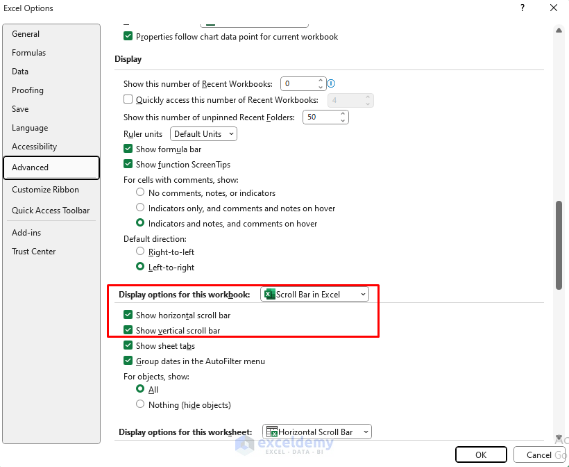
Select File and go to Options to open the Options dialog.
Select the Advanced option feature and scroll down to Display options for this workbook section.
Uncheck the options for the scroll bars (marked in the image below). If you want to hide one of the scroll bars, just uncheck that.
Click OK.

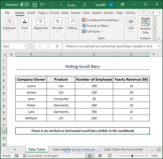
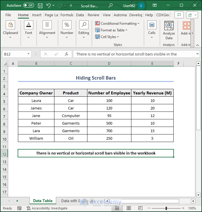
You can see that there are neither the horizontal scroll bar nor the vertical scroll bar.

How to Resize the Horizontal Scroll Bar in Excel?

Drag the three-dot icon beside the horizontal scroll bar in the Excel sheet right or left. If you move this icon to the left, the scroll bar size will increase. Otherwise, it will decrease.

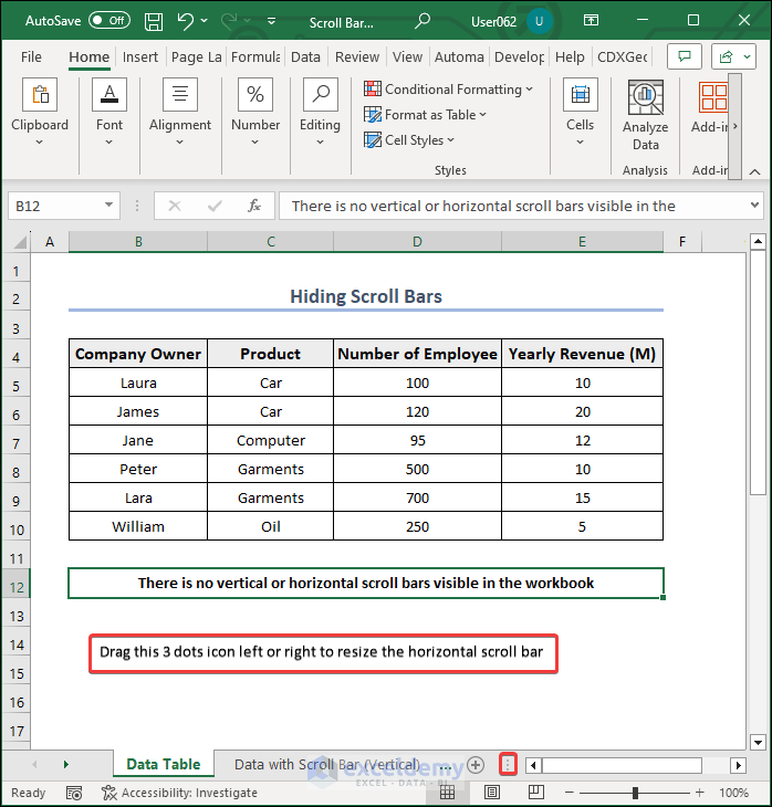
We dragged the icon to the left so the size of the horizontal scroll bar increased. See the image below.

How to Fix a Missing Scroll Bar (Default) in Excel?

One reason for missing Scroll Bars can be that users may disable them in the workbook. To enable them, select File and go to Options and scroll down to Display options for this workbook.
Make sure to check Show horizontal scroll bar and Show vertical scroll bar.
You will see the Scroll Bars appear.

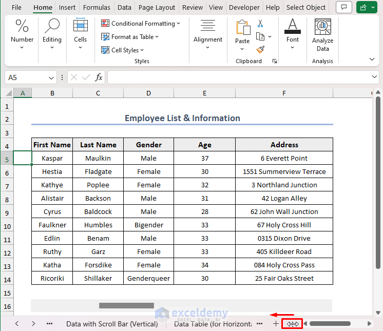
There is another reason why the Horizontal Scroll Bar may be missing. See the image below.

Drag the marked icon to the left, and you will see the Horizontal Scroll Bar.

Things to Keep in Mind

To modify or interact with the scroll bar, ensure that you are in Design Mode. It allows you to edit the Scroll Bar
Make sure to set the appropriate range and value limitations for the Scroll Bar to ensure it covers the desired range of values and behaves as intended.
It’s essential to thoroughly test the Scroll Bar’s functionality, especially if it interacts with other elements or data in your Excel workbook. Validate that it works as expected under various scenarios.

Frequently Asked Questions

Is it possible to control the scroll bar using VBA in Excel?

Yes, you can use VBA to control the scroll bar. You can programmatically scroll to a certain location by using the Scroll method, or you can alter the position of the Scroll Bar by adjusting the Value property.

What is the purpose of the SmallChange and LargeChange properties of a scroll bar in Excel?

When you click the arrow buttons on the scroll bar, the SmallChange property determines the incremental value, but the LargeChange property determines the incremental value when you click on the Scroll Bar’s track area.

Is it possible to hide or disable a scroll bar in Excel?

You can hide or disable a scroll bar. To do so, right-click on the Scroll Bar, select Format Control, and then check or uncheck the Display as icon option in the Control tab to hide or show the Scroll Bar. You can disable the Scroll Bar by setting the Enabled value to False in VBA.

Scrollbar in Excel: Knowledge Hub

<< Go Back to Excel Parts | Learn Excel

Get FREE Advanced Excel Exercises with Solutions!