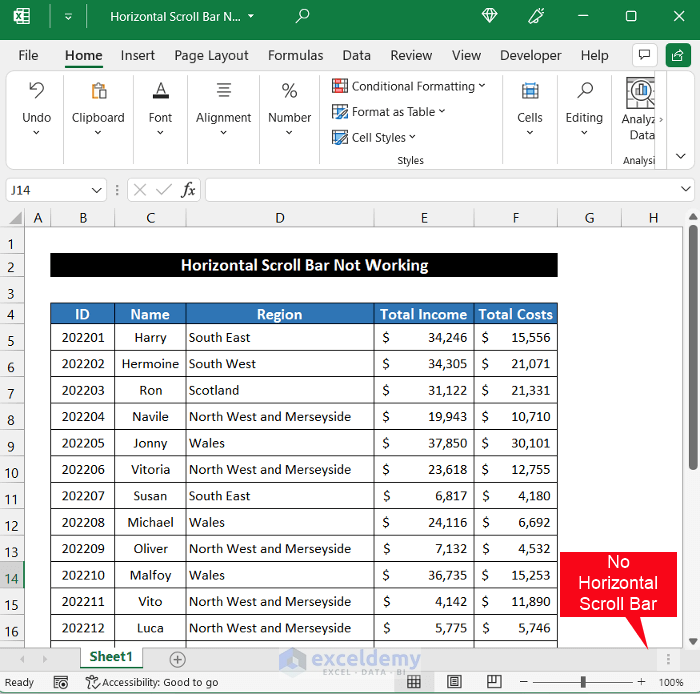
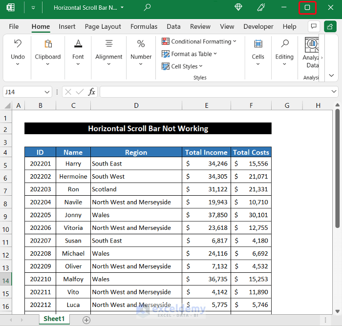
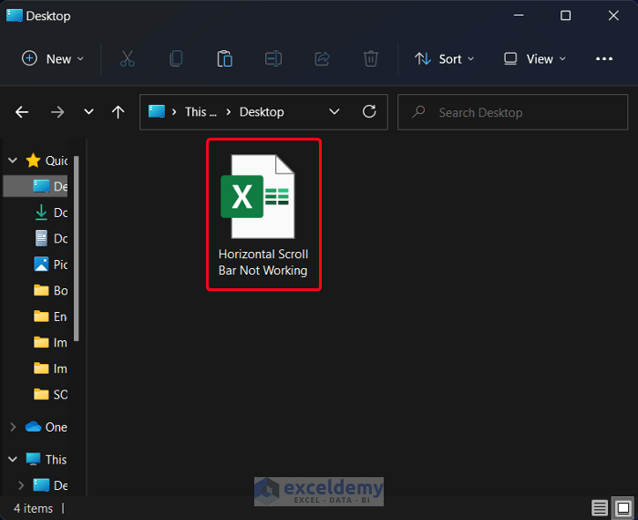
Consider a dataset of 21 employees. We mentioned their ID in column B, their names in column C, residency area in column D, total income in column E, and total costs in column F. Our Horizontal Scroll Bar of Excel is not working for the dataset.
Solution 1 – Modify Excel Options
Steps:
- Select File and choose Options.
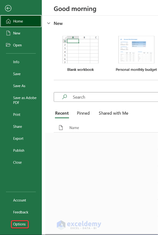
- The Excel Options dialog box will appear.
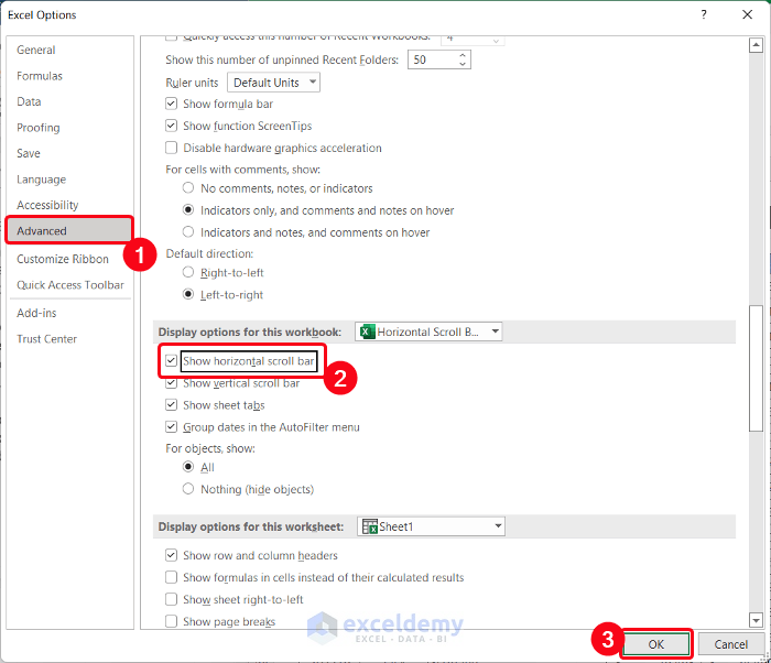
- Choose the Advanced tab.
- Scroll down to the Display options for this workbook section.
- Check the Show horizontal scroll bar option and click OK.
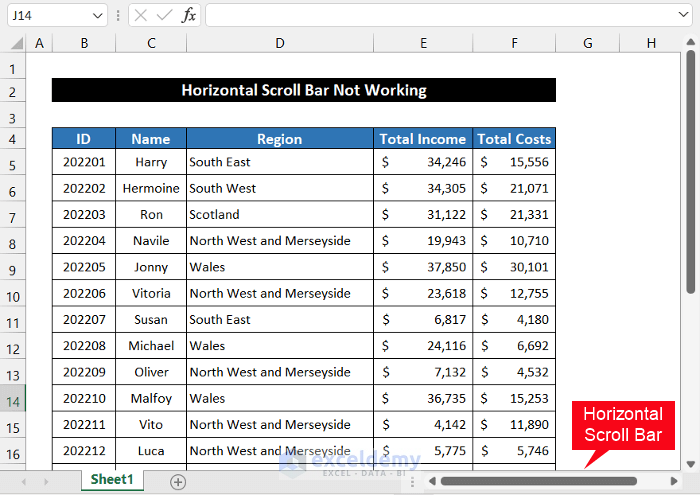
- You will get the Horizontal Scroll Bar in your Excel sheet.
Read More: [Solved!] Scroll Bar Not Working in Excel
Solution 2 – Maximize the Excel Window
Steps:
- Click on the Maximize button to get the full-screen view of the Excel window.
- The Horizontal Scroll Bar should appear at the bottom of the Excel spreadsheet.
Read More:[Fixed!] Bottom Scroll Bar Missing in Excel
Solution 3 – Extend the Horizontal Scroll Bar
Steps:
- Move your cursor through the Sheet Tab.
- At the bottom-right corner, the cursor should convert into a resize icon, as shown in the image.
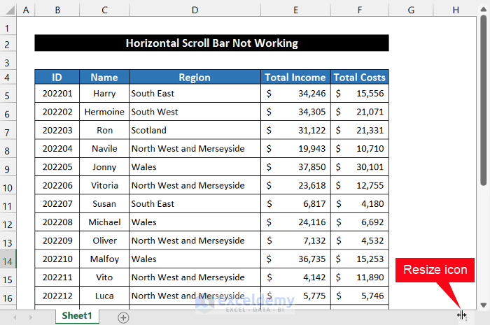
- Click and drag to the left.
- You should see the Horizontal Scroll Bar expand.
Read More: [Fixed!] Excel Scroll Bar Too Long
Solution 4 – Check the Scroll Bar Automatic Hiding Option
Steps:
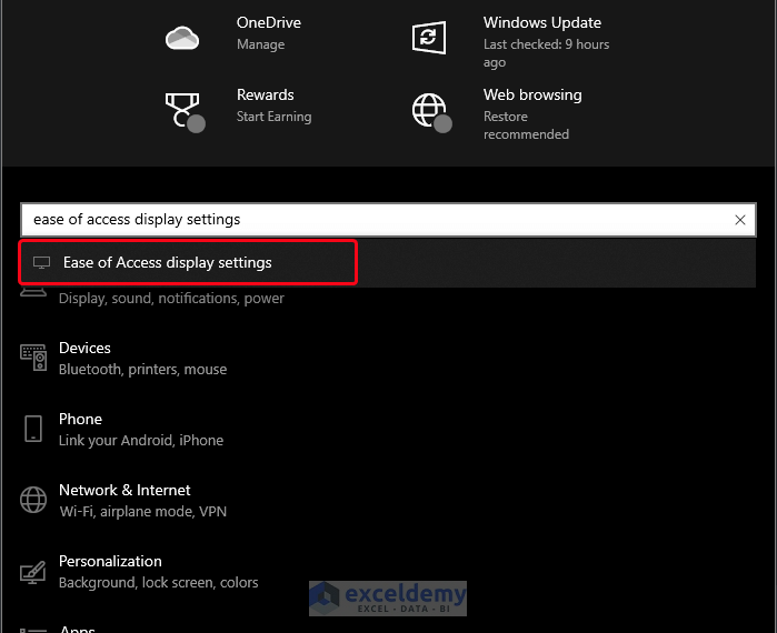
- Click on the Start button on your computer or press the Windows button on your device.
- Select the Settings option.
![]()
- Go to Ease of Access of Display in the Search Engine.
- Click on the Automatically hide scroll bars in Windows option.
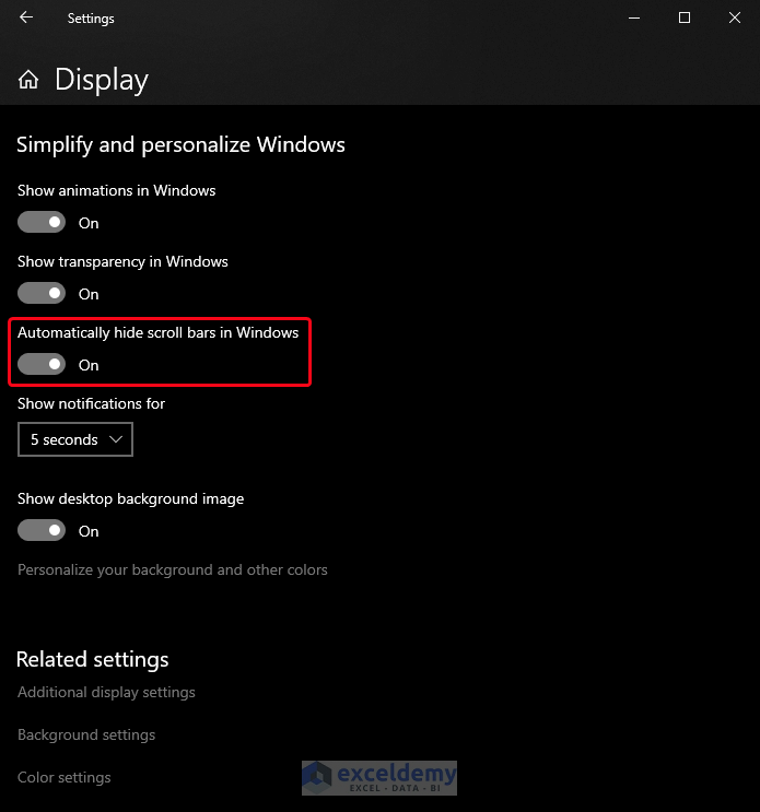
- Close the Settings window.
- Open Microsoft Excel, and you will get the scroll bar.
Read More: [Solved]: Excel Scroll Bar Moves but Sheet Does Not
Solution 5 – Use the Tiled Option from the Arrange All Command in View Tab
Step:
- In the View tab, select the Arrange All option from the Window group.
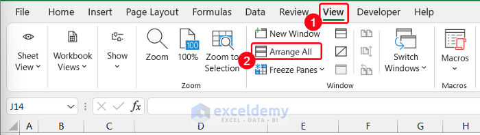
- A small dialog box called Arrange Windows will appear.
- Select the Tiled option and click OK.
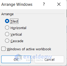
- You will get the Horizontal Scroll Bar at the bottom of your Excel window.
Solution 6 – Unfreeze Panes
Steps:
- In the View tab, select the drop-down arrow of the Freeze Panes option from the Window group.
- Click on the Unfreeze Panes option.
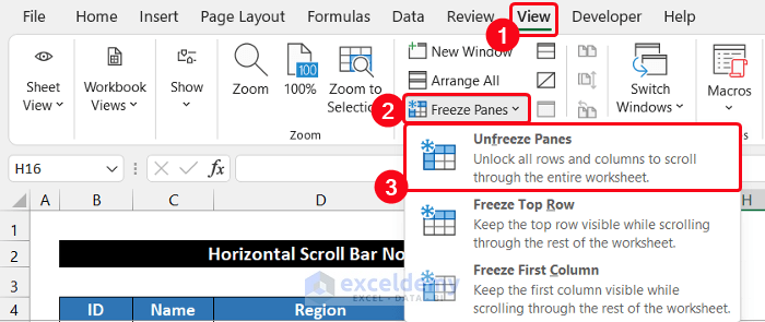
- You will get the Horizontal Scroll Bar at the bottom of the window.
Solution 7 – Close and Re-Open Excel
Steps:
- Click on the Close button.
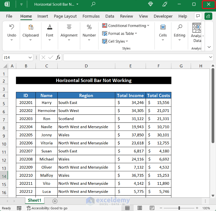
- Double-click on your desired file to re-open it.
- The scroll bar might start working.
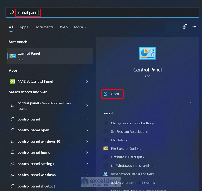
Solution 8 – Re-Install Microsoft Office
Steps:
- Click the Search Engine on the Taskbar.
- Search for Control Panel and open it.
- Click on the Uninstall a program option.
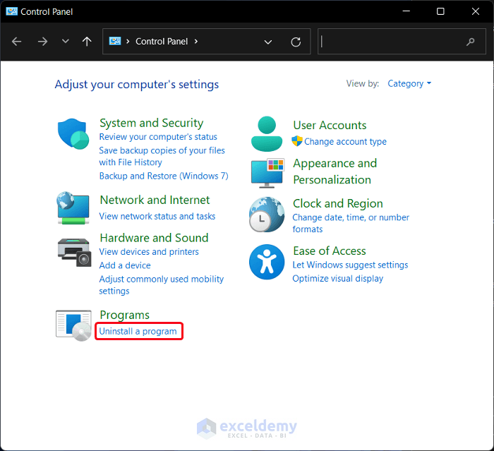
- The Programs and Features dialog box will appear.
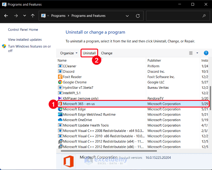
- Scroll down to Microsoft-365en or something similar.
- Select the application and click Uninstall. It will take a while to uninstall the program.
- Double-click on the OfficeSetup.exe file to re-install the application and follow the instructions. You can get the file from the official Excel website.
- The default settings for the horizontal bar should make it appear.
Download the Practice Workbook
<< Go Back to Scrollbar in Excel | Excel Parts | Learn Excel
Get FREE Advanced Excel Exercises with Solutions!

Mine stopped working, but only when I hide cells to the right of the data. I can delete those cells, but when I hide specifically column AE (my last column with data is in column Z) the scroll bar locks to the far left. I can still move around using arrows and it will move the screen, but if I touch that bar it goes to the far left and won’t stop.
I thought it might be an issue with the notes, as it was refusing to hide the columns and the workbook went all the way to column C~~ (somewhere past the 2028th column). I deleted the notes and replaced them with comments, and it lets me hide anything now (and my workbook doesn’t go past column AE unless I tell it to), but now I have this scroll issue (the issue happens only when I hide column AE). Maybe the notes get “saved” at column C~~, and comments get “saved” 5 columns to the right of your data?
Hello Timmy C.
It sounds like Excel may still be recognizing something far to the right of your visible data, which can affect how the horizontal scroll bar behaves. Even if your actual data ends at column Z, hidden objects, formatting, comments, or other elements can extend the used range of the worksheet.
You can try a few things to fix it:
1. Check for objects or formatting to the right
Press Ctrl + End to see where Excel thinks the last used cell is.
If it jumps somewhere far to the right (like column CXX or beyond), Excel is still detecting content there.
2. Clear unused columns
Select the first empty column after your real data (AA or AB, depending on your sheet).
Press Ctrl + Shift + Right Arrow to select all columns to the end.
Right-click and choose Delete (not just Clear Contents).
3. Save and reopen the workbook
After deleting the extra columns, save the file, close Excel, and reopen it. This resets the worksheet’s used range in many cases.
4. Check for hidden objects
Go to Home → Find & Select → Go To Special → Objects to see if any shapes, comments, or notes are placed far to the right.
Regarding Notes vs. Comments, they normally shouldn’t extend the scroll range by themselves, but if a note or object was accidentally placed far off to the right, Excel might treat that area as part of the used sheet, which can lead to scroll bar issues like the one you described.
If the problem still occurs specifically when column AE is hidden, it may indicate that AE contains some formatting or an object tied to that column. Clearing or deleting columns beyond your actual data usually resolves this.
Regards,
ExcelDemy