How to Insert Scroll Bar in Excel (2 Suitable Methods)

Q: How do I enable scrolling in Excel?

Select the File tab and then click Options > Advanced. Then, select the Show horizontal scroll bar and the Show vertical scroll bar checkboxes under Display options for this workbook and click OK.

Here is an overview of how to insert a scroll bar in the Excel worksheet using the Developer tab.

2 Ways to Insert Scroll Bar in Excel

There are two types of scroll bars in Excel:

Form Control Scroll Bar
ActiveX Control Scroll Bar

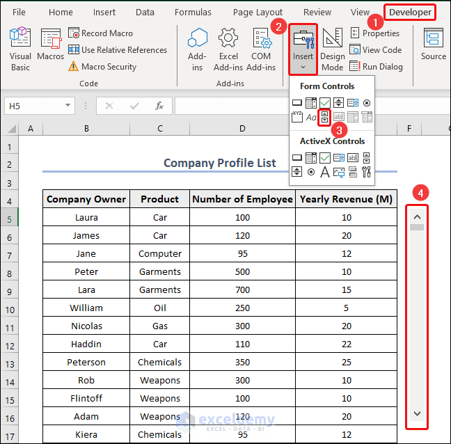
Method 1 – Inserting a Scroll Bar from Form Controls

Select Developer, then go to Insert and the Form Controls group, then choose Scroll Bar.
Hold the left mouse button and move the cursor horizontally or vertically to insert the scroll bar in the worksheet.

How to Use a Scroll Bar in Excel

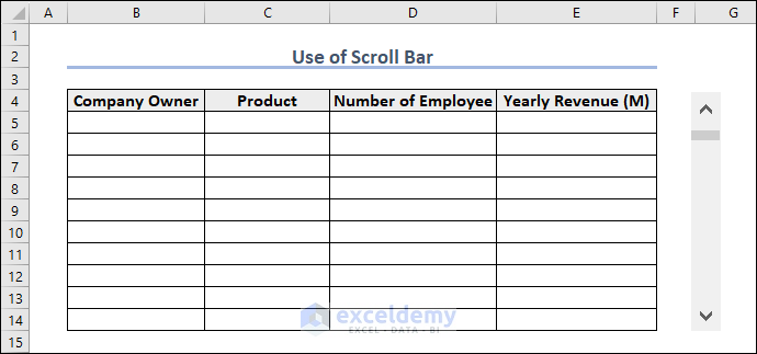
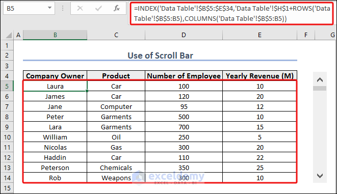
In the sheet named Data Table, we have a dataset of 30 rows in the range B5:E34. 10 of them will be visible by the scroll bar.

Company Owner	Product	Number of Employee	Yearly Revenue (M)
Laura	Car	100	10
James	Car	120	20
Jane	Computer	95	12
Peter	Garments	500	10
Lara	Garments	700	15
William	Oil	250	5
Nicolas	Gas	300	20
Haddin	Car	110	22
Peterson	Chemicals	350	25
Rob	Weapons	300	10
Flintoff	Weapons	100	10
Adam	Weapons	120	20
Kiera	Chemicals	95	12
Jason	Chemicals	500	10
Ashish	Car	250	22
Hiran	Car	300	25
Dushan	Car	110	10
Joy	Computer	350	10
Kane	Garments	700	10
Beer	Garments	650	15
Mike	Weapons	100	10
Gray	Weapons	120	10
Tison	Chemicals	95	20
Erikson	Chemicals	500	12
Nicles	Car	350	10
Brek	Car	700	10
Drek	Computer	650	15
Laren	Oil	300	20
Jovan	Gas	110	22
Flintar	Car	350	25

Open a new sheet or choose another area in the worksheet.
Insert the same column headings of your original dataset.
Insert a scroll bar.
Right-click on the scroll bar and select Format Control.
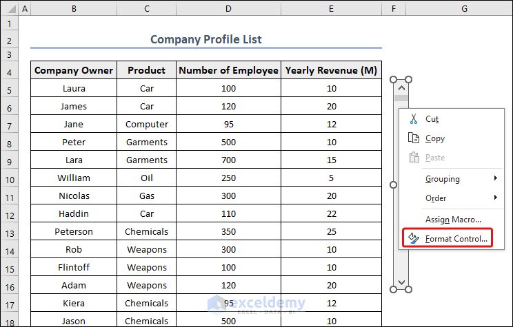
The Format Control dialog box will appear.
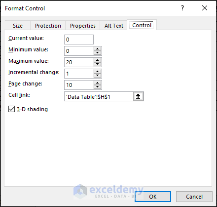
In the Format Control dialog box, set up the following:
- - Minimum Value: 0
  - Maximum Value: 20 (as we have 30 rows and we want to show 10 rows at a time, making the scroll bar value 20 will show the rows 21-30)
  - Incremental Change: 1
  - Page Change: 10
  - Cell Link: ‘Data Table’!$H$1 (H1 cell of the Data Table sheet)
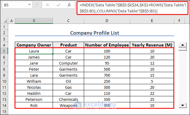
To extract data from the original table to the new sheet, copy this formula into the first cell under the first column:
=INDEX('Data Table'!$B$5:$E$34,'Data Table'!$H$1+ROWS('Data Table'!$B$5:B5),COLUMNS('Data Table'!$B$5:B5))
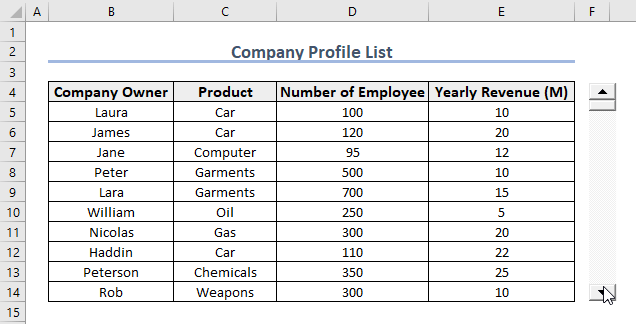
The B5:E34 range is in the Data Table sheet. In this sheet, the H1 cell is linked to the scroll bar. The content of the B5 cell of the Data Table should appear in the new table’s B5 cell after applying the formula. You can also use the formula below instead of using the INDEX function: =OFFSET('Data Table'!B5,'Data Table'!$H$1,0,1,1)
Drag the Fill Handle icon down up to 10 rows and to the right to autofill the data table.

The scroll bar is ready for application.

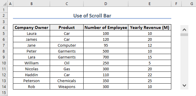
Thus, you can efficiently use a scroll bar in Excel.

Note

Here is a short description of the Control values:

Current value: This value refers to the position of the scroll box in the scroll bar. If the scroll box is on the top, the value becomes 0. If it’s at the bottom of the scroll bar, the value becomes equal to the Maximum value. And keeping it at the bottom of the scroll bar makes the Current value equal to the Maximum value. Each time you scroll up or down, the Current value changes from minimum to maximum value. You can see this change in the linked cell.
Minimum value: This will be the value of the linked cell when the scroll box is at the top.
Maximum value: This will be the value of the linked cell when the scroll box is at the bottom.
The area of the visible data table by the scroll bar can be maintained by the minimum and maximum values. So you need to set them properly.
Incremental change: This value determines the step amount each time you scroll up or down. Say you set the Minimum value and Incremental change to 0 and 2 respectively. If you keep clicking the scroll-down button, the value of the Current value will be 0, 2, 4, 6, and so on.
Page change: This is the amount the scroll bar value changes when you click on the scroll bar track.
Cell link: The scroll bar generates values while it’s triggered (scroll up or down). So a cell needs to be linked with the scroll bar to store these values. The linked cell contains the Current values of the scroll bar corresponding to the position of the scroll box. The values can be used in a formula to control the scroll bar.

Read More: How to Adjust Scroll Bar in Excel

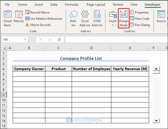
Method 2 – Inserting a Scroll Bar from ActiveX Control

Select the Developer tab and go to Insert, then select Scroll Bar from the ActiveX Controls box.
Hold the left mouse button and move the cursor horizontally or vertically to insert the scroll bar in the worksheet.
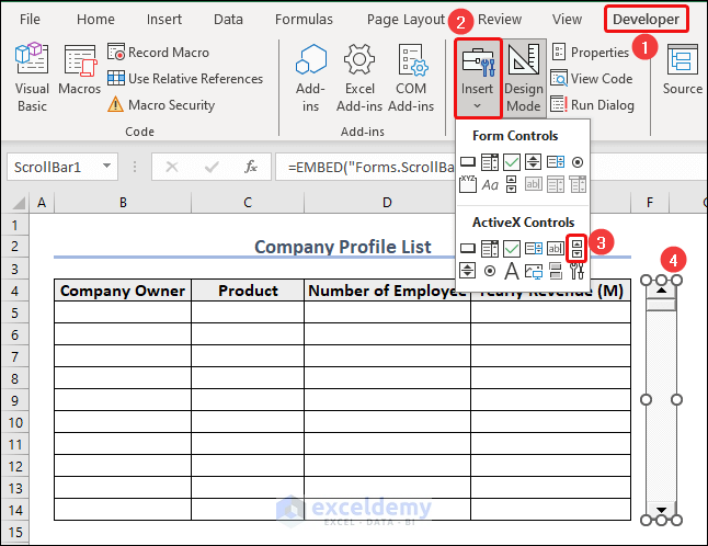
Select Properties from the Controls group.
In the Properties window, select a linked cell and choose Max and Min values.
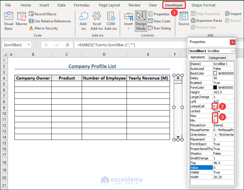
Cell K1 of the Data Table sheet is the linked cell, Max and Min values are 20 and 0, respectively.
Disable the Design mode just by clicking on the button.
Use the formula below and apply the Fill Handle like the previous method:
=INDEX('Data Table'!$B$5:$E$34,$K$1+ROWS('Data Table'!$B$5:B5),COLUMNS('Data Table'!$B$5:B5))

The scroll bar is ready.

Download the Practice Workbook

Insert Scroll Bar.xlsm

Frequently Asked Questions

How do I enable scrolling in Excel?

Select the File tab and then click Options > Advanced. Then, select the Show horizontal scroll bar and the Show vertical scroll bar checkboxes under Display options for this workbook and click OK.

How do I remove a scroll bar in Excel?

To remove a scroll bar from the worksheet, right-click on the scroll bar to select the scroll bar and press the “Delete” key on your keyboard.

Can I customize the appearance of the scroll bar?

To customize the appearance of the scroll bar created from the Form Controls group, right-click on the scroll bar, choose “Format Control,” and make adjustments in the Format Control dialog box. Moreover, you have a wide range of options to format the scroll bar if you create it from the ActiveX Controls group. Just go to its Properties and modify the necessary parameters or appearance.