How to Add a Scroll Bar to a Chart in Excel - 6 Steps

Q: How do I set up a dynamic range for my chart using a scroll bar?

Define a range of data and use formulas that incorporate the value from the linked cell (controlled by the scroll bar) to determine the dynamic range for your chart. This can be achieved using OFFSET, INDEX, or other relevant functions.

This is an overview.

Step 1 – Create an Excel Chart from the Dataset

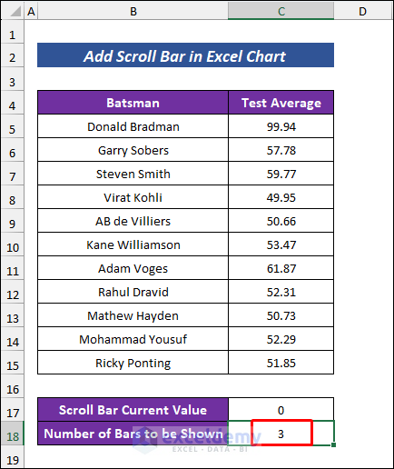
Select the whole data.
Go to the Insert tab and choose a chart.

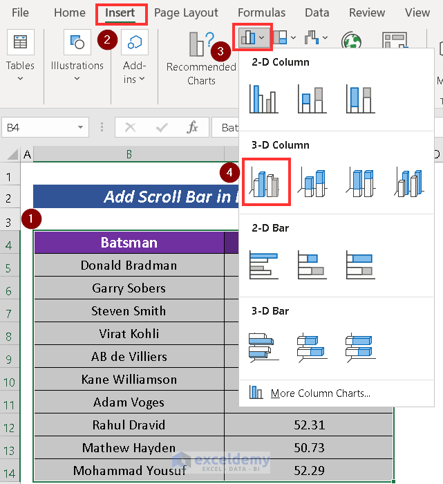
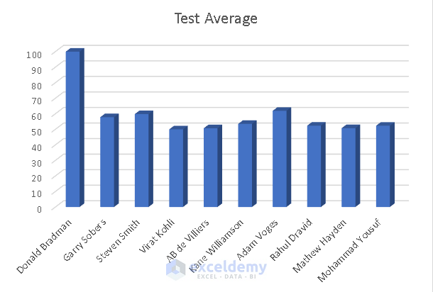
The chart is created:

Step 2 – Insert a Scroll Bar

Select Developer and click Insert.
Choose Scroll Bar in Form Controls.
Drag the cursor to create the scroll bar under the chart.

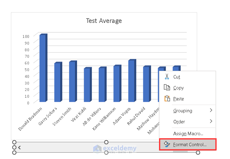
Step 3 – Customize the Scroll Bar

Right-click.
Select Format Control.
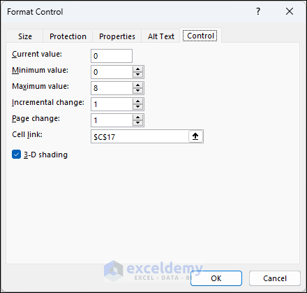
In the Format Control dialog box, set up the parameters:
- Minimum Value: 0
- Maximum Value: 8 (there are 11 bars and you want to show 3 bars at a time: the scroll bar value 11 will show bars 9-11)
- Incremental Change: 1
- Page Change: 1 (if you click the scroll bar area, the scroll box will move 1 step at a time)
- Cell Link: $C$17
- Click OK.

Step 4 – Create Named Ranges Using Formulas and Linked Cell Values

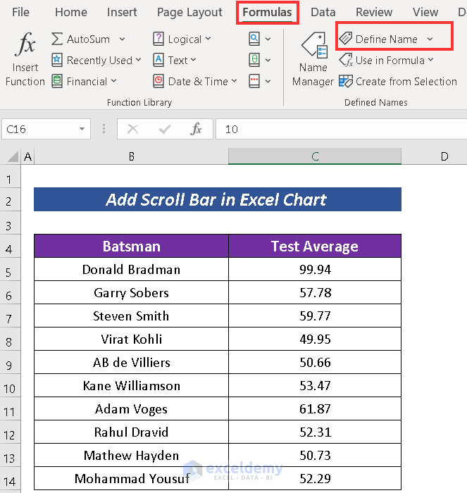
Define how many bars will be visible in the chart.
Select Formulas > Define Name.
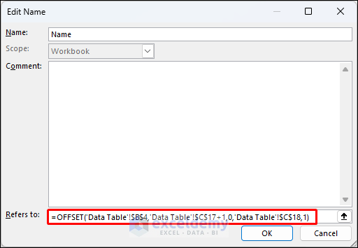
In the Edit Name dialog box:
Name the range.
Use the following formula in ‘Refers to‘ to define the value in B5: B14:

=OFFSET('Data Table'!$B$4,'Data Table'!$C$17+1,0,'Data Table'!$C$18,1)The formula uses the OFFSET function which defines a partial dynamic range from B5:B14. The linked cell (‘Data Table’!$C$17) provides the number of rows of the partial range. The height of the range is set by the cell reference ‘Data Table’!$C$18.

Click OK.
Use the following formula in the ‘Refers to’ with the name Average to define C5:C14:

=OFFSET('Data Table'!$C$4,'Data Table'!$C$17+1,0,'Data Table'!$C$18,1)The OFFSET function evaluates the values in C5 till the end of the table, ignoring other values.

Step 5 – Modify the Data Range in the Chart Using the Named Ranges

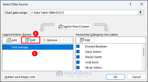
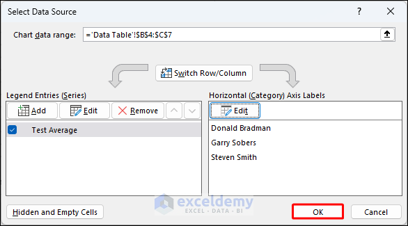
Right-click the chart and choose Select Data.
In Select Data Source, select the column heading in Legend Entries (Series) and go to Edit.
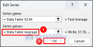
In the Edit Series dialog box:
- Enter the reference of the column heading in Series name.
- Use the named range for numeric data (Average) in Series values.
Click OK.
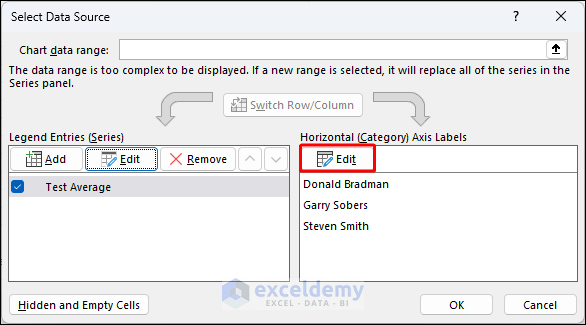
Click Edit in Horizontal (Category) Axis Labels.
Use the named range for names (Name) in Axis label range and click OK.
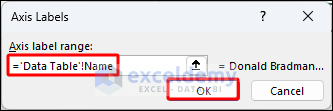
Click OK in the Series Data Source dialog box.

Step 6 – Use the Scroll Bar in the Chart

Using this Scroll Bar, you will see 3 vertical bars out of 11 in the chart. Observe the GIF.

You see three vertical bars each time you scroll.

Download Practice Workbook

Adding Scroll Bar.xlsx

Frequently Asked Questions

Can I use multiple scroll bars in one chart?

Yes, you can use multiple scroll bars to control different aspects of your chart, such as axis ranges or data series. Each scroll bar should be linked to a different cell.

How do I set up a dynamic range for my chart using a scroll bar?

Define a data range and use formulas that incorporate the value in the linked cell (controlled by the scroll bar) to determine the dynamic range. Use the OFFSET, INDEX, or other functions.