In this article, we will describe how to create a vertical scroll bar in Excel.
What Is a Scroll Bar in Excel?
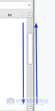
A scroll bar is a slider that enables us to view data in Excel from left to right or top to bottom. We can view data incrementally by clicking on the direction signs at the sides of a scroll bar. We can also drag the scroll bar to directly navigate from top to bottom or left to right.
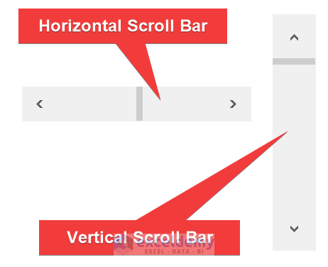
There are two types of scroll bars in Excel:
- Vertical Scroll Bar: Enables us to view data from top to bottom.
- Horizontal Scroll Bar: Enables us to view data from left to right.
Why Use a Vertical Scroll Bar in Excel?
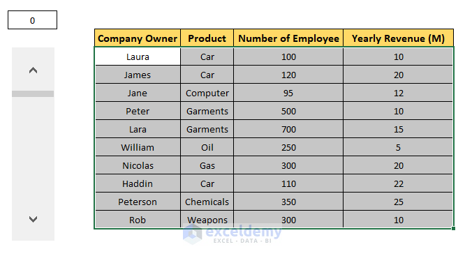
Here we have a long data table that goes down to row 34. The whole data table can’t be viewed on the screen at the same time. With 100% zoom, only up to row 29 is visible.
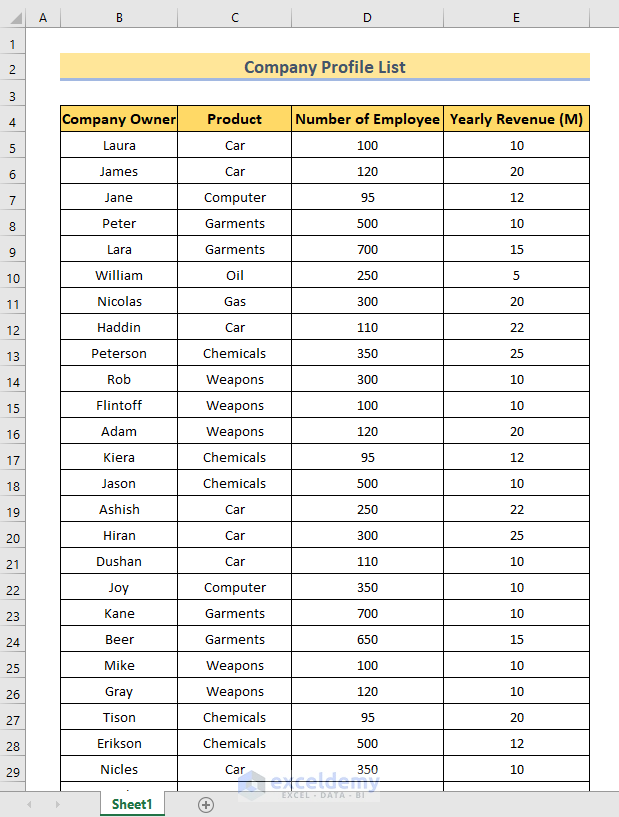
To see the rest of the rows of the data table, we’ll have to scroll down manually using the mouse scroll button, which is inconvenient.
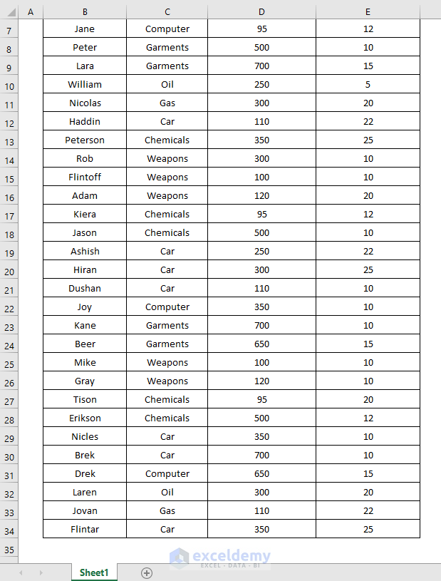
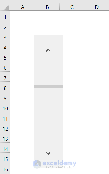
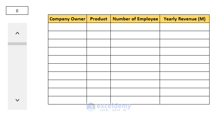
Instead, we can attach a vertical scroll bar like the one below. Now all of the data in the data table can be viewed just by controlling the vertical scroll bar, and without affecting the display of anything else on the screen.
Let’s create a vertical scroll bar like this one.
How to Create a Vertical Scroll Bar in Excel
Scroll bars can be accessed from the Form Controls group, which is located in the main ribbon of the Developer tab.
Step 1 – Adding the Developer Tab
The Developer tab is disabled by default. If you can see the Developer tab on your ribbon, it is enabled, and you can skip the this step.
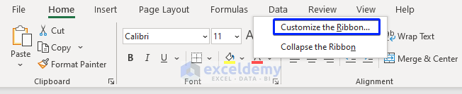
- Right-click anywhere on the Home tab.
A pop-up dialog box will appear.
- Select Customize the Ribbon from the dialog box.
This will open the Excel Options dialog box.
- Select Customize Ribbon from the left side of the Excel Options dialog box.
- Check the Developer option in the Main Tabs box.
- Click OK.
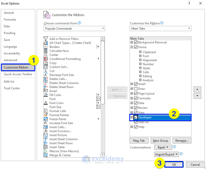
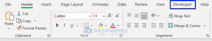
The Developer tab is added to the main ribbon between the View and the Help tabs.
Step 2 – Draw and Create a Vertical Scroll Bar
Now let’s create the vertical scroll bar in the Excel sheet.
- Go to the Developer tab.
- Click on the Insert drop-down menu.
- From the Form Controls group, select Scroll Bar (Form Control).
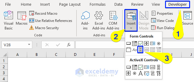
You will see a plus icon (‘+’) on your Excel sheet.
- Draw a vertical bar by dragging the plus icon (‘+’) using the left-click button of your mouse.
When you release the left-click button of your mouse, the vertical bar you just drew turns into a vertical scroll bar.
Step 3 – Tweaking the Format Control Dialog Box for the Vertical Scroll Bar
Next, we’ll activate the vertical scroll bar.
- Right-click on the vertical scroll bar.
- Select Format Control from the context menu.
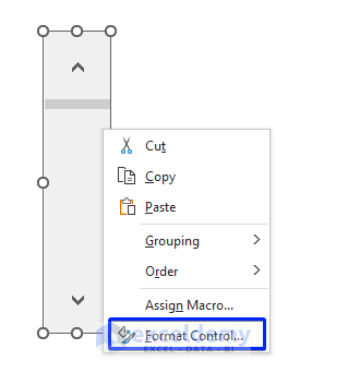
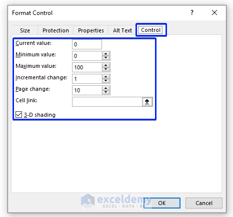
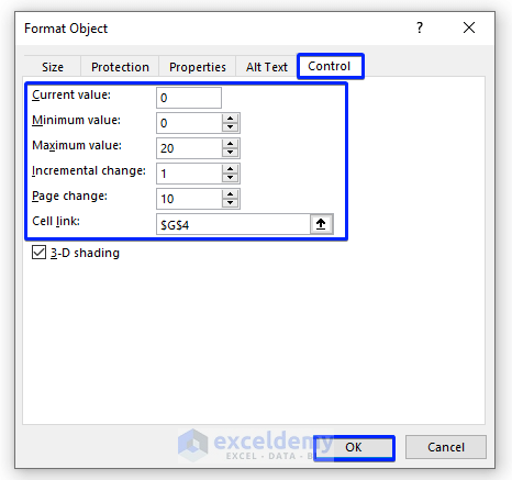
The Format Control dialog box will appear with the Control tab pre-selected.
There are several options to set:
- Current value
- Minimum value
- Maximum value
- Incremental change
- Page change
- Cell link
Besore we set them, let’s discuss how these options affect the scroll bar.
How Does a Vertical Scroll Bar Work?
The vertical scroll bar is tied to a cell with a numerical value. The value in the cell and how it will change are determined by the Format Control dialog box.
When you click on the vertical scroll bar, the value of the cell increases or decreases depending on which side of the scroll bar is clicked.
Then a lookup formula tied to the cell is used to retrieve data from the source dataset. When the value of the cell changes, the lookup formula extracts different values responding to these changes.
With that in mind, here is what the parameters of the Format Control dialog box mean:
Current value: The initial value of the linking cell, which depends on your dataset.
Minimum value: The Minimum value should be equal to the Current Value or 0.
Maximum value: Maximum value is the highest value that the vertical scroll bar can have.
Incremental change: Determines the dataset update rate. Using 1 will update the dataset by 1 row each time you click on the scroll bar, and so on.
Page change: Determines how many rows to update at a time when you drag the vertical scroll bar vertically.
Cell link: The cell address where the value corresponding to the vertical scroll bar is stored.
Let’s set these parameters in the Format Control box.
Read More: How to Insert Scroll Bar in Excel
Calculating Maximum Value
The Maximum Value is very sensitive. If you set it wrong, you will get the #REF! error.
We can use the ROWS function to determine the Maximum Value.
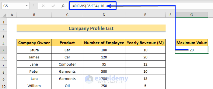
- Choose any blank cell and insert the following formula:
=ROWS(B5:E34)-10Here, B5:E34 is the range of the dataset, and 10 is the number of rows to show at a time. The ROWS function calculates the total number of rows in the range B5:E34.
- Press ENTER.
The Maximum Value will be returned.
- Now set the options as follows:
- Current value: 0
- Minimum value: 0
- Maximum value: 20
- Incremental change: 1
- Page change: 10
- Cell link: $G$4
- After setting all the values, click OK.
Check the vertical scroll bar values. Now, the minimum value is set to 0 and the maximum value is 20.

Step 4 – Retrieve Data & Add a Formula to Activate the Vertical Scroll Bar
Now we’ll connect the vertical scroll bar with the dataset.
- Copy the formats of your dataset and paste them next to the vertical scroll bar.
Since the Page Change value is set to 10, we’ve taken 10 rows in total here.
- Insert the following lookup formula, which consists of the INDEX, ROWS & COLUMNS functions, in the first cell of the blank dataset:
=INDEX($B$5:$E$34,$G$4+ROWS($B$5:B5),COLUMNS($B$5:B5))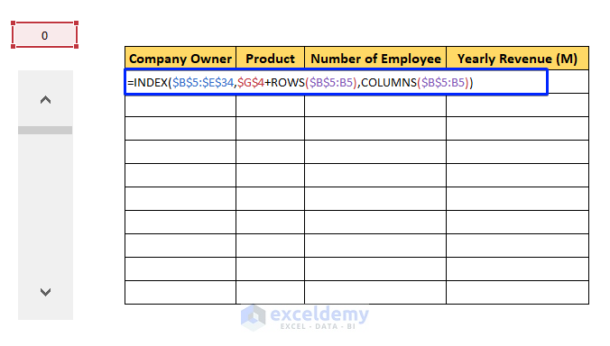
Formula Breakdown
- COLUMNS($B$5:B5): The COLUMNS function calculates the total number of columns in the range $B$5:B5. In the range, the first cell address is absolute but the second cell is not. So, when you drag the formula, it will expand. The total number of columns in the source data table is returned.
- ROWS($B$5:B5): The ROWS function calculates the total number of rows in the range $B$5:B5. In the range, the first cell address is absolute but the second cell is not. So, when you drag the formula, it will expand. A serial number starting from 1 is returned. According to this serial number, the INDEX function will retrieve specific rows from the source data table.
- $G$4+ROWS($B$5:B5): The range in the ROWS function will expand up to $B$5:B14, a maximum of 10. The source data table has a total of 30. To retrieve all the rows, $G$4 is added to the result of ROWS($B$5:B5). Cell $G$4 contains a number ranging from 0 to 20. So adding $G$4 to ROWS($B$5:B5) can produce up to 30. This means the formula can retrieve all the rows from the source data range, $B$5:$E$34.
- $B$5:$E$34: The data range of the source data table.
- INDEX($B$5:$E$34,$G$4+ROWS($B$5:B5),COLUMNS($B$5:B5)): The INDEX function pulls specific rows specified by $G$4+ROWS($B$5:B5) and specific columns specified by COLUMNS($B$5:B5) from the range $B$5:$E$34.
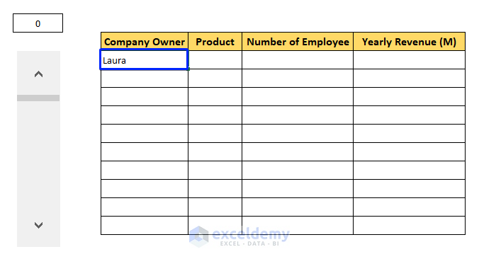
- Press ENTER.
Laura will be displayed in the cell where the formula was applied.
- Drag the lookup formula down and across the blank data table that you created earlier using the Fill Handle.
We have created a vertical scroll bar and connected it with a secondary data table.
Now, clicking the vertical scroll bar will cause the data in the data table to change like in the following animation.
Read More: How to Adjust Scroll Bar in Excel
Show & Hide the Default Vertical Scroll Bar in Excel
Excel has a built-in vertical scroll bar located on the right side of the Excel window.
By sliding this vertical scroll bar, you can also scroll up or down through the data table.
This built-in vertical scroll bar can be hidden or shown. Here’s how to do it.
Method 1 – Using Advanced Options
Steps:
- Go to the File tab.
- Select Options.
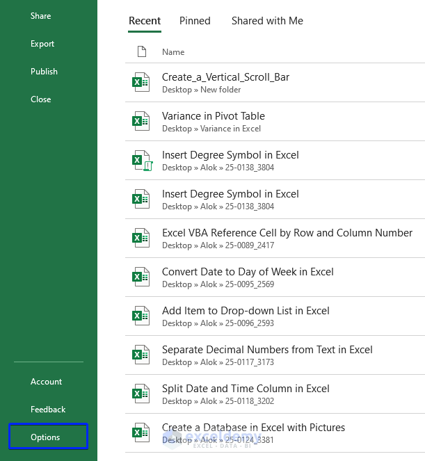
The Excel Options dialog box will open.
To hide the vertical scroll bar:
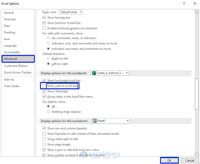
- Select Advanced.
- Uncheck ‘Show vertical scroll bar’ under the Display options for this workbook section.
- Click OK.
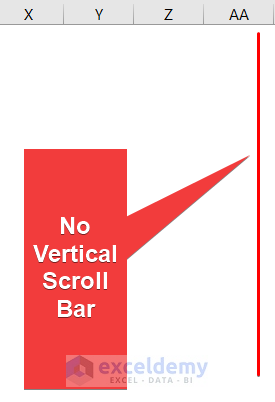
The vertical scroll bar in the spreadsheet has vanished.
To show the vertical scroll bar:
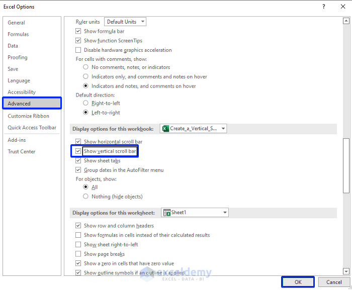
- Select Advanced in the Excel Options dialog box.
- Check ‘Show vertical scroll bar’ under the Display Options for this workbook section.
- Click OK.
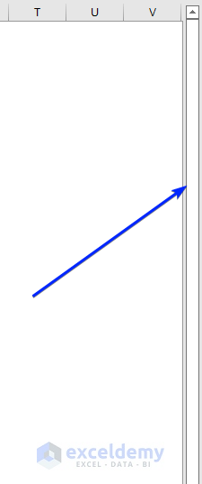
The built-in vertical scroll bar is visible again.
Method 2 – Using VBA
Steps:
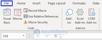
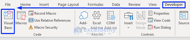
- Go to the Developer tab and select Visual Basic from the Code group. Or press ALT + F11.
This will open the Visual Basic Editor.
- Select the Insert tab.
- Choose Module from the drop-down menu.
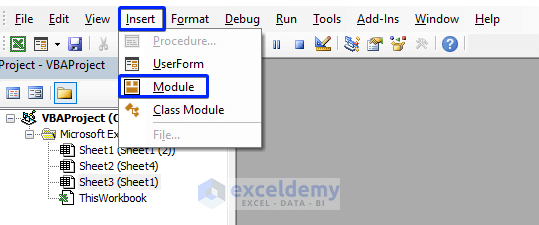
A new module will open.
To hide the built-in vertical scroll bar:
- Copy the VBA code below.
- Paste it in the VBA Editor.
- Save the code.
- Press F5 to run the code.
Option Explicit
Private Sub Hide_Vertical_Scroll_Bar()
With ActiveWindow
.DisplayVerticalScrollBar = False
End With
End Sub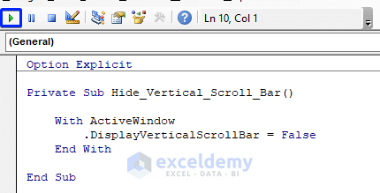 The vertical scroll bar has disappeared.
To show the built-in vertical scroll bar:
- Copy the VBA code below.
- Paste it in the VBA Editor.
- Save the code.
- Press F5 to run the code.
Option Explicit
Private Sub Show_Vertical_Scroll_Bar()
With ActiveWindow
.DisplayVerticalScrollBar = True
End With
End Sub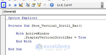 The vertical scroll bar is visible again.
Related Articles
<< Go Back to Scrollbar in Excel | Excel Parts | Learn Excel
Get FREE Advanced Excel Exercises with Solutions!
