If you’re looking for quick and easy ways to use comma in Excel formula, this article will be helpful. While working with Excel, we often need to add a comma in our data set to represent our data properly. In this article, we are going to learn 2 practical and easy-to-use ways to use comma in Excel formula.
Importance of Using Commas in Excel
We frequently run into situations in Excel where we need to add a comma to our data set. It can be representing numerical data in accounting forms or adding comma between texts etc. Doing this by hand can be tiresome work. But Excel has some slick tricks up its sleeve to help you in this regard.
In this section of the article, we’ll go through some practical approaches to using commas in Excel formulas in detail.
Not to mention that we have used Microsoft Excel 365 version for this article, you can use any other version according to your convenience.
1. Using Comma in Excel Formula for Numbers
In the beginning, we will learn how we can use comma in Excel formula for numbers. We will discuss 3 different methods of doing it. They are described below.
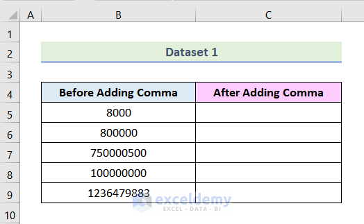
In the following dataset, we have some numbers under the Before Adding Comma column. Here no comma is added to the numbers. Our goal is to add comma to the numbers properly.
1.1 Using TEXT Function
Using the TEXT function is one of the most effective ways to use comma in Excel formula. Let’s follow the steps mentioned below to do it.
Steps:
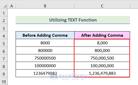
- Firstly, go to cell C5 and insert the following formula in cell C5.
=TEXT(B5,"#,##0")Here, cell B5 represents the cell of column Before Adding Comma. The “#,##0” is the format to add a comma after every 3 numbers.
- Then press ENTER.

Subsequently, you will get the following output.

By using Excel’s AutoFill feature, we can get the rest of the outputs as marked in the following picture.
Read More: How to Add Thousand Separator in Excel Formula
1.2 Applying Comma Style Feature in Excel
Applying Comma Style is another efficient method to use comma in Excel formula. Let’s learn the following steps.
Steps:
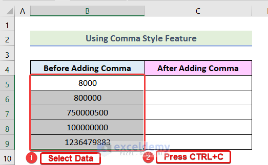
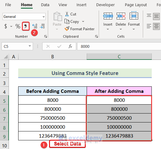
- Firstly, select the cells of the column of Before Adding Comma.
- After that, press CTRL + C to copy the cells.
- Now, click on cell C5 and press CTRL + V to paste the copied cells.
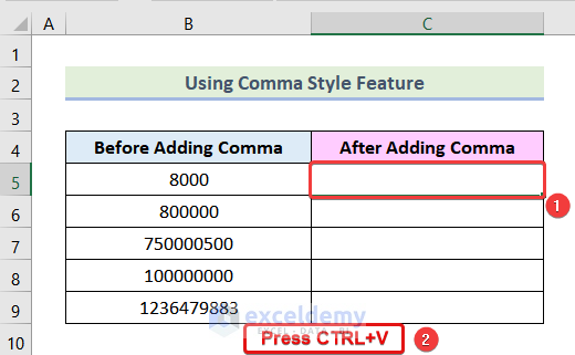
Afterward, you will see that the cells have been pasted like the following image.

- Then, select the cells of the column After Adding Comma.
- Following that, click on the Comma Style icon as marked in the image given below.
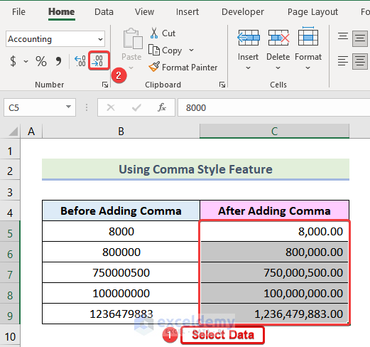
Consequently, you will see that commas are added to the cells like in the following picture.

If you want to remove the decimal places then follow this simple step.
- Select the cells of the column After Adding Comma.
- Afterward, click on the Decrease Decimal icon as shown in the following image.
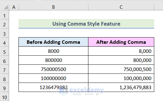
As a result, you will get the following output on your worksheet.
1.3 Applying Cell Formatting to Use Commas in Excel Formula
Utilizing Cell Formatting is one of the easiest methods to use comma in Excel formula. Let’s follow the steps mentioned below.
Steps:
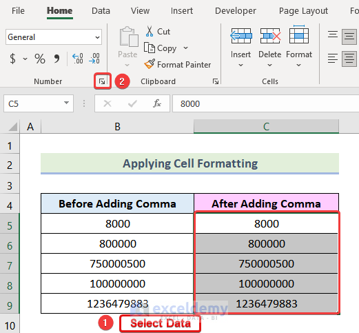
- By using the previously mentioned steps, we will copy and paste the cells of the column Before Adding Comma.
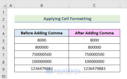
- After that, select the cells of the column After Adding Comma.
- Following that, click on the Clipboard icon as marked in the image given below.
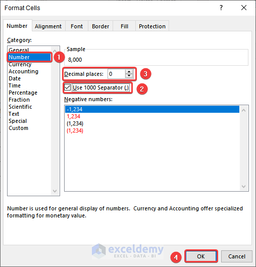
Consequently, a Format Cells dialogue box will open like the following image.

Note: You can just press CTRL + 1 to open the Format Cells option.
- Now, choose Number from the dialogue box.
- After that, check the box of Use 1000 Separator (,).
- If you want to remove Decimal Places, then decrease Decimal Places to 0.
- Finally, click on OK.
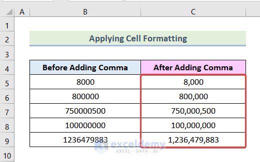
There you go! You have successfully used comma in Excel formula.
Read More: How to Apply Excel Number Format in Thousands with Comma
2. Using Comma in Excel Formula for Texts
In this section of the article, we are going to learn how to use commas in Excel formulas for Texts.
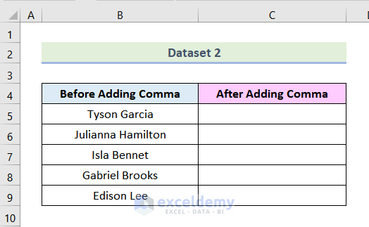
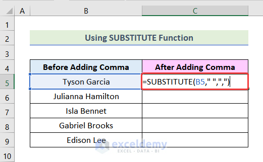
In the following dataset, we have the names of several people in the Before Adding Comma column. Our goal is to add comma between the two words.
2.1 Using SUBSTITUTE Function
Using the SUBSTITUTE function is one of the most popular ways to use comma in Excel formula for texts. Let’s learn the steps mentioned below to do this.
Steps:
- Firstly, go to cell C5 and insert the following formula.
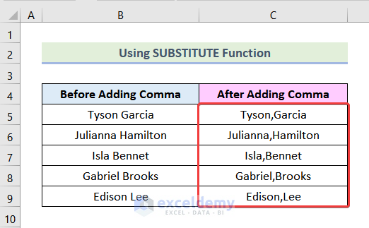
=SUBSTITUTE(B5," ",",")- After that, hit ENTER.
Consequently, a comma will be added between two texts like the following image.

We can get the rest of the data by using Excel’s AutoFill feature.
Read More: How to Add Comma in Excel Between Names
2.2 Combining REPLACE and FIND Functions to Use Comma in Excel Formula
Applying REPLACE and FIND functions is another effective way to use comma in Excel formula. Let’s follow the steps given below.
Steps:
- Firstly, go to cell C5 and enter the formula given below.
=REPLACE(B5,FIND(" ",B5,1),1,",")Formula Breakdown
- Here, B5 is the text we want to replace.
- FIND(” “,B5,1) denotes the starting position from where will start replacing.
- “ “ indicates the text we want to find. In this case, it is space.
- B5 represents the in which text we want the space.
- 1 denotes the starting position of the search.
- 1 represents the number of characters we want to replace.
- “,” denotes the new text that will replace the old one.
- After that, press ENTER.
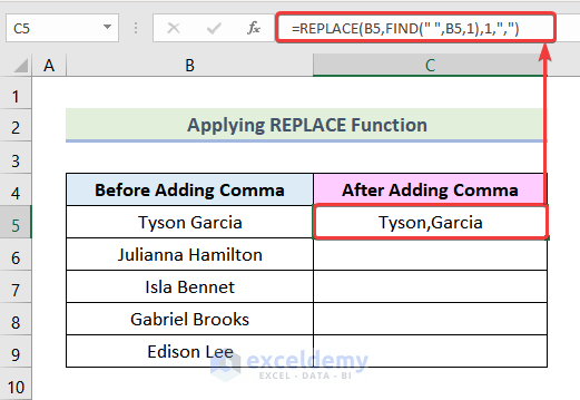
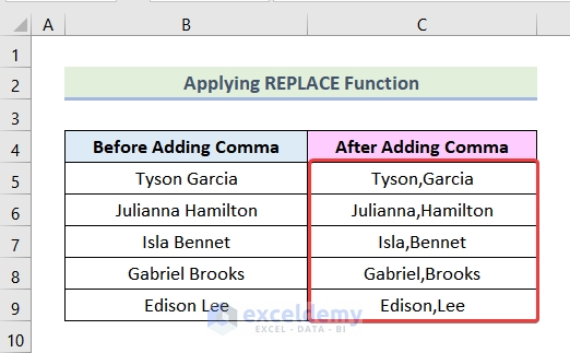
Consequently, you will get the following output.

By using the AutoFill feature of Excel, we can get the rest outputs like the image given below.
2.3 Using Commas in a List
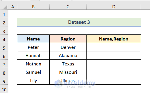
In the following dataset, we have the Name and Region of some people. Our aim is to represent them together using a comma between them using an Excel formula.
2.3.1 Adding a Single Comma
To add a comma between the Name and the Region, we will follow the steps mentioned below.
Steps:
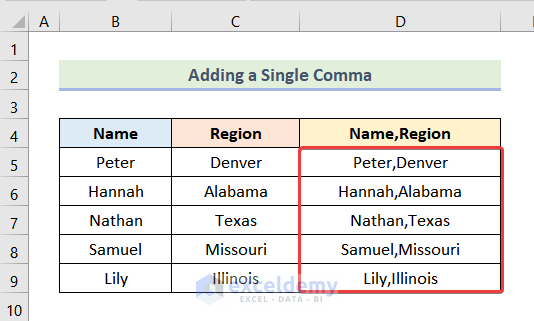
- Firstly, enter the following formula in cell D5.
=B5&","&C5Here cell B5 represents the cell of the Name column and cell C5 indicates the cell of the Region column.
- After that, press ENTER.

Subsequently, you will see that a comma is added between the Name and the Region as shown in the following image.

Using Excel’s AutoFill feature will provide us with the rest of the outputs.
2.3.2 Introducing Comma by Using TEXTJOIN Function
Using the TEXTJOIN function is one of the easiest ways to use comma in Excel formula. The steps to do this are mentioned below.
Steps:
- Firstly, go to cell D5 and enter the following formula.
=TEXTJOIN(",",TRUE,B5,C5)Formula Breakdown
- Here, “,” is the delimiter that we will use.
- TRUE means we will ignore_empty
- B5 and C5 are 1st Text and 2nd Text that will be joined.
- Afterward, hit ENTER.
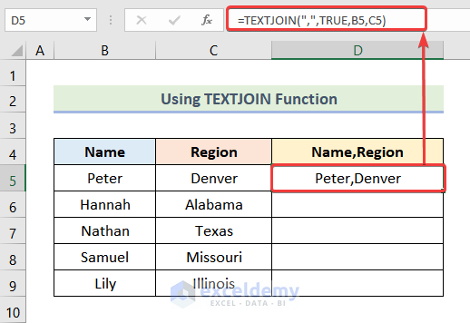
Consequently, you will see the following image on your screen.

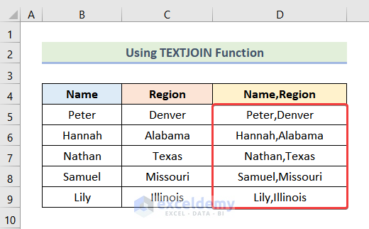
Using Excel’s AutoFill feature will give the rest of the output as shown in the picture given below.
2.3.3 Adding Comma by Using CONCATENATE Function
Another efficient method to use comma in Excel formula is by using the CONCATENATE function. Let’s follow the steps given below.
Steps:
- Firstly, use the following formula in cell D5.
=CONCATENATE(B6,",",C6)Here, B6,”,”,C6 are the texts that we want to join together.
- Then, press ENTER.
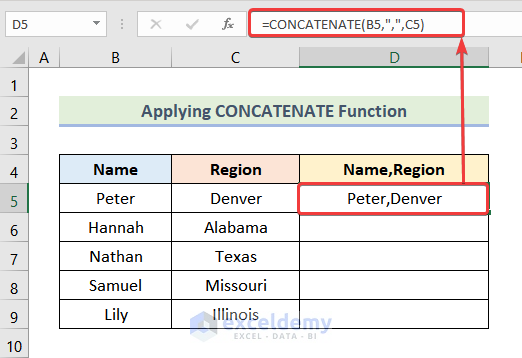
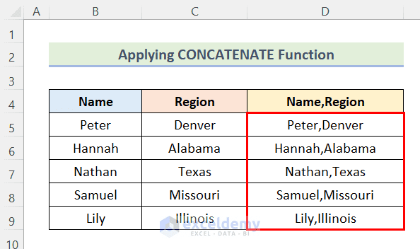
Consequently, you will get the following output on your worksheet.

Now, to get the rest of the data, we will use Excel’s AutoFill feature.
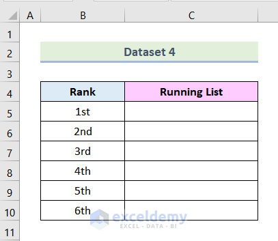
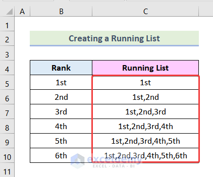
2.3.4 Creating a Running List with Comma
We can create a running list by using comma in Excel formula. In the following dataset, we have the rank of 1st 6 people in a race. Our goal is to create a running list by using comma in Excel formula.
Steps:
- Firstly, write 1st in cell C5.
Here, cell C5 indicates the cell of the Running List.
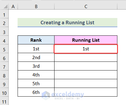
- After that insert the following formula in cell C6.
=C5&","&B6Here, cell B6 represents the cell of the Rank.
- Following that, hit ENTER.

Consequently, you will get the following output.

By using Excel’s AutoFill feature, we can get the rest of the outputs as marked in the following image.
2.4 Using Comma in Excel Formula to Split String
In Excel, we can use comma to split strings. Now, we are going to learn how we can do that.
In the following dataset, we have 5 strings consisting of the name, region, and age of some people. We will try to separate the name, region, and age from the string.
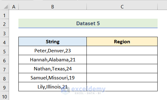
2.4.1 Applying MID and FIND Function to Split String
Applying the MID function and the FIND function is a simple way to split strings using comma. Firstly, we will split the region from the string. To do this, we will follow the steps mentioned below.
Steps:
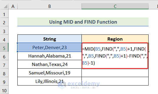
- Firstly, go to cell C5 and enter the following formula.
=MID(B5,FIND(",",B5)+1,FIND(",",B5,FIND(",",B5)+1)-FIND(",",B5)-1)Formula Breakdown
- Here, FIND(“,”,B5)+1 indicates the starting position of the 1st character after the 1st comma.
- FIND(“,”, B5, FIND(“,”, B5)+1) represents the initial position of the 1st character after the 2nd comma.
- -FIND(“,”,B5)-1 indicates that all the characters after the 2nd comma in the string, are omitted.
- After that, hit ENTER.
Subsequently, we will get the Region as output.

Using Excel’s AutoFill feature will give us the rest of the regions as shown in the image given below.

Read More: How to Add a Comma Between City and State in Excel
How to Use Correct Regional List Separator in Excel
In Excel, List Separator varies with the location of the user. For example, in the United States, and United Kingdom the List Separator sign is Comma (,). On the other hand, in Germany, and France the List Separator sign is Semicolon (;). In this section of the article, we will learn how we can change the List Separator based on the respective region.
Using the Windows Settings option is a straightforward way to correct the regional List Separator in Excel. Let’s follow the steps mentioned below.
Steps:
- Firstly, go to the Search Box in the Taskbar of your computer and type intl.cpl.
- After that, press ENTER.

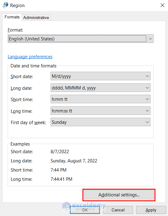
- Subsequently, the Region dialogue box will open, and click on the marked potion as shown in the image given below.

- Following that, select English (United States) from the list.
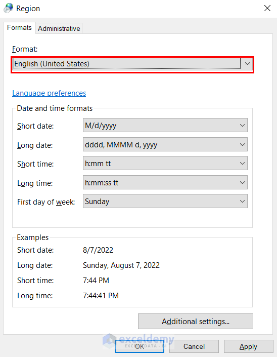
- Next, click on the Additional settings.
- After that, you will see that your List Separator is changed according to the location you chose.
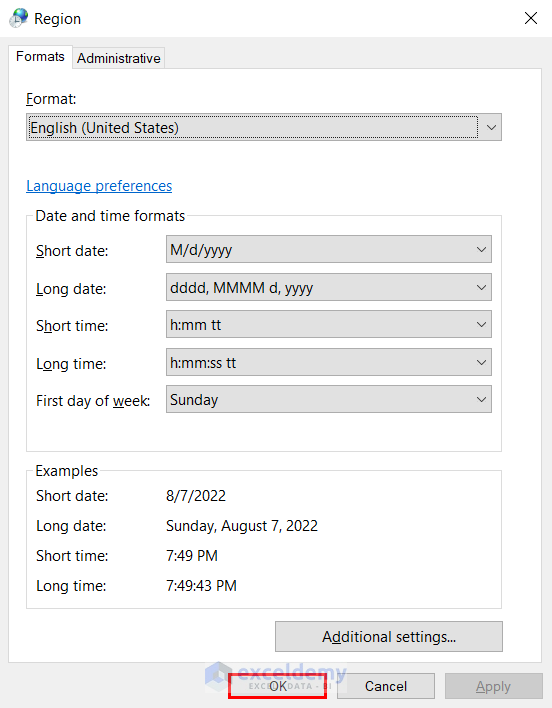
- Then click OK.

- Following that, click on Apply from the Region dialogue box.
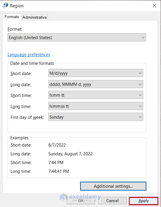
- Finally, click on OK.
How to Enable System Separators in Excel
Utilizing Excel’s Options feature is an efficient way to enable system separators in Excel. The steps necessary to do this are discussed below.
Steps:
- Firstly, go to the Files tab from the Ribbon.
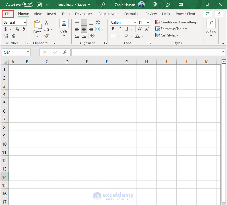
- After that, select the Options.

Consequently, the Excel Options dialogue box will open in your worksheet like the following image.
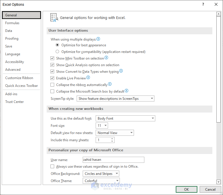
Note: To open the Excel Options dialogue box, you can use the keyboard shortcut ALT + F + T.
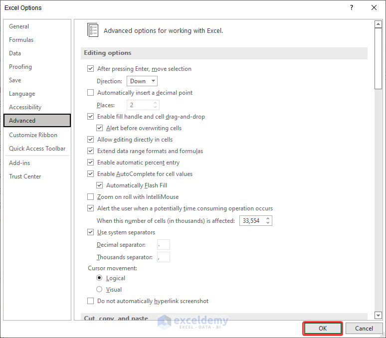
- Next, go to the Advanced tab from the Excel Options dialogue box.

- Now, check the box of Use system separators.
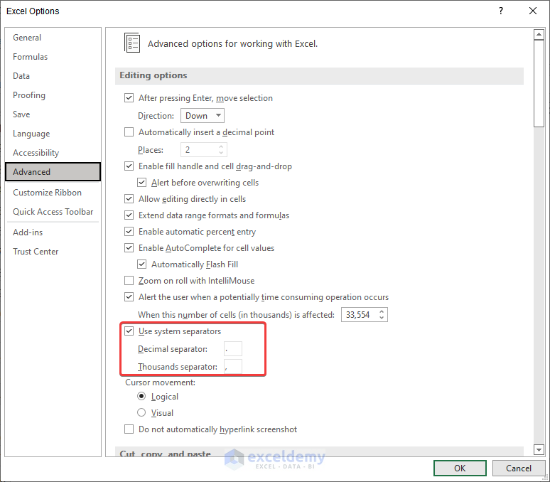
- Finally, click OK.
Download Practice Workbook
Conclusion
Finally, we have to the end of the article. I sincerely hope that this article was able to guide you to use comma in Excel formula. Please feel free to leave a comment if you have any queries or recommendations for improving the article’s quality. Happy learning!
Related Articles
- How to Add Comma in Excel at the End
- How to Add Comma Before Text in Excel
- How to Insert Comma in Excel for Multiple Rows
<< Go Back to How to Add Comma in Excel | Concatenate Excel | Learn Excel
Get FREE Advanced Excel Exercises with Solutions!
