How to Sort Column Chart in Descending Order in Excel

Get FREE Advanced Excel Exercises with Solutions!

Column chart is one of the most powerful tools for visualizing data in Excel. But sometimes, we need to change the order of our dataset into ascending or descending order for a clear understanding of the chart. There are several ways to sort column chart in descending order. In this article, we will guide you on how to sort column chart in descending order in excel with 3 useful methods.

Table of Contents hide

Download Practice Workbook

3 Useful Methods to Sort Column Chart in Descending Order in Excel

1. Apply Sort Tool to Create Column Chart in Descending Order

2. Sort Column Chart in Descending Order with Excel Pivot Chart

3. Apply Excel Formulas to Sort Column Chart in Descending Order

Conclusion

Download Practice Workbook

Download this sample file to try by yourself.

Sort Column Chart in Descending Order.xlsx

3 Useful Methods to Sort Column Chart in Descending Order in Excel

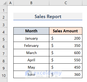
To describe the methods, we prepared a sample dataset with the information on Sales Amount in the months of January-June in cell range B4:C10.

Let us create a column chart first out of this dataset.

First, go to the Insert tab and select Insert Column or Bar Chart from the Charts section.

Then, select 2-D Clustered Column from the drop-down menu.

That’s it, we have our required column chart.

As you can see the bars are not in descending order according to values. Therefore, follow the methods below to sort this column chart in descending order.

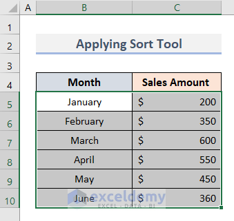
1. Apply Sort Tool to Create Column Chart in Descending Order

In this first method, we will use the Sort tool in excel for reordering the column chart.

First, select cell range B5:C10.

Then, go to the Home tab and click on Sort & Filter under the Editing group.

Afterward, select Custom Sort from the drop-down section.

Now, in the Sort window, change the category in Sort by section.
Also, change the Order as Largest to Smallest.

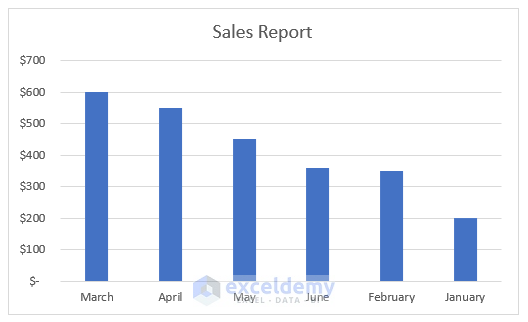
Finally, you will see that the column chart is changed to descending order automatically.

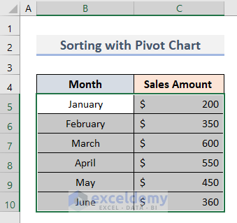
2. Sort Column Chart in Descending Order with Excel Pivot Chart

The pivot chart is another helpful method to sort the column chart in descending order. To do the task, follow the steps carefully.

In the beginning, select cell range B5:C10.

Then, go to the Insert tab and click on PivotChart under the Charts group.

Following, select PivotChart from the drop-down section.

Next, select the Location where you want to insert the Pivot Chart.
As we want to get it beside our dataset, so provided cell E4 as the Location.

Then, press OK.
Now, place the Data Fields as per the image in the PivotChart Fields.

Therefore, you will get the initial column chart.
After this, click on the field button on the bottom left of the chart.

Afterward, select More Sort Options from the Context Menu.

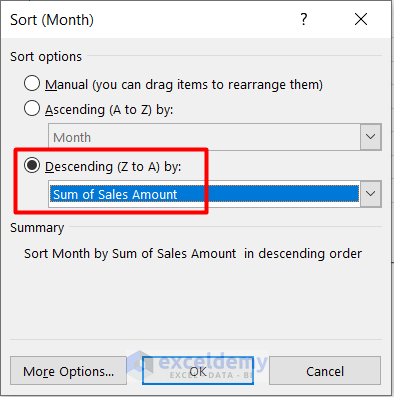
Lastly, select the category in the Descending (Z to A) by section and hit OK.

Finally, you will get the required descending-ordered column chart.

Similar Readings

3. Apply Excel Formulas to Sort Column Chart in Descending Order

In this last section, we will apply some excel formulas for reordering column chart into descending order. Let’s see how it works.

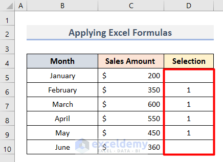
Firstly, create a new column titled Selection beside the dataset.
In this new column, type 1 beside the cells that you want to insert in the chart.

Then, create another table for the new dataset.

Now, insert this formula in cell F5.

=FILTER(B5:B10,D5:D10=1)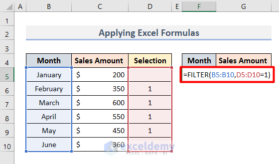

Then, press Enter and you will see the cells that we chose earlier from the dataset in cell range F5:F8.

Here, the FILTER function allows filtering cell range B5:B10 based on the criteria range D5:D10.

Next, type this formula in cell F5 to change the Month names into descending order according to their values.

=SORTBY(FILTER(B5:B10,D5:D10=1),FILTER(C5:C10,D5:D10=1),-1)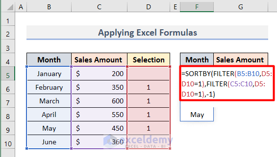

Here, the SORTBY and FILTER functions sort and filter the contents of cell range B5:B10 and C5:C10 based on their corresponding array in cell range D5:D10. Along with it, as we denoted the Selection as 1, each filtered cell is equal to 1.

Afterward, press Enter and you will see the Month names’ order is changed to descending order based on values.

After this, insert this formula to get the adjacent values of the months.

=VLOOKUP(F5#,B5:C10,2,FALSE)

In this formula, the VLOOKUP function finds the value of cell F5 and onwards from the cell range B5:C10. As the adjacent values are in the 2nd column, therefore we typed 2 as the column reference. Finally, type FALSE for an exact match.

Lastly, insert the Column Chart as we described previously.
That’s it, you will get the chart in descending order.

To cross-check the formula, type 1 in cell D10 to insert its adjacent cell’s value into the new table.
Accordingly, you will see that the table automatically rearranges in descending order.

Finally, insert a Column Chart like before to get the descending-ordered chart.

Conclusion

Concluding this article, I hope you will find it helpful how to sort column chart in descending order in excel with 3 useful methods. Try them with the sample file. Follow ExcelDemy for more tutorials.

How to Sort Column Chart in Descending Order in Excel

Download Practice Workbook

3 Useful Methods to Sort Column Chart in Descending Order in Excel

1. Apply Sort Tool to Create Column Chart in Descending Order

2. Sort Column Chart in Descending Order with Excel Pivot Chart

3. Apply Excel Formulas to Sort Column Chart in Descending Order

Conclusion

Related Articles

Leave a reply Cancel reply