How to Create a Variable Width Column Chart in Excel

A variable width column chart portrays data in a more convenient way as the columns correspond to the values in the dataset, unlike a simple column chart. Unfortunately, up until now, there is no such chart type in Excel. Therefore you need to follow workarounds to do that until Excel adds this chart type. This article will help you to do that. You will also be able to create a Marimekko (Mekko) chart in Excel by following this article.

How to Create a Variable Width Column Chart in Excel: 4 Steps

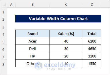
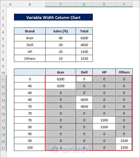
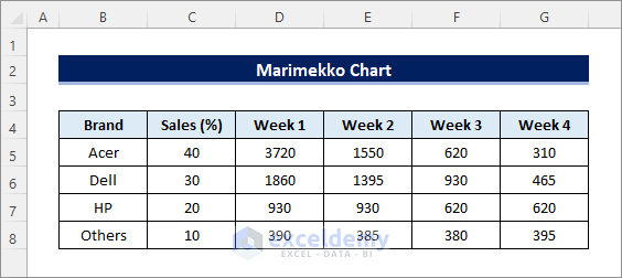
Assume you have the following dataset showing the market shares of various PC brands and the total sales within a month. The sale percentages add up to 100%. You need to create a column chart with this dataset where the widths of the columns correspond to the values.

Follow the steps below to be able to do that.

Step 1: Make a Duplicate Table

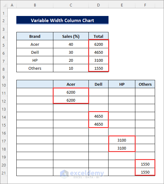
First, create a duplicate table with an empty column at the beginning and a single column for each Brand. Then copy the Brand names and paste them as Transpose to create column Headers. Next, copy each sale amount twice in the respective columns in a way that the first sale amount is copied to the first two rows and there is a blank row between two different brand sales as shown below.

Step 2: Input Cumulative Sales Percentages

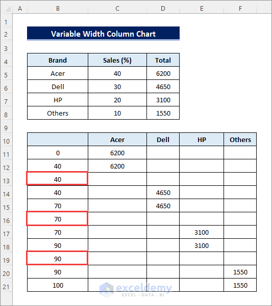
Now you need to type the cumulative sales percentages in the first blank column. For Acer, it starts from 0 and ends at 40. For Dell, it starts from 40 and ends with 40+30=70. For HP, it starts from 70 and ends with 70+20=90. For Others, it starts with 90 and ends with 90+10=100.

Notice that the cells adjacent to the blank cells in the first column have the same values. So type the same values as the adjacent cells (40, 70, 90) in those blank cells respectively as shown below.

Step 3: Apply the Paste Special Feature

Now you need to fill all other blank cells in the table with 0. Select the table except for the first column and go to Home >> Find & Select >> Go to Special >> Blanks >> OK. This will select all blank cells within the selection.

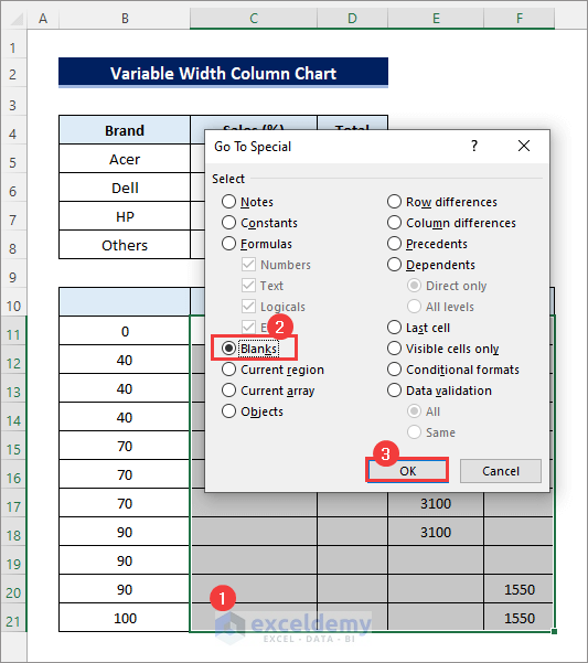
Then type 0 and press CTRL + ENTER to replace the blank cells with zeros as shown below.

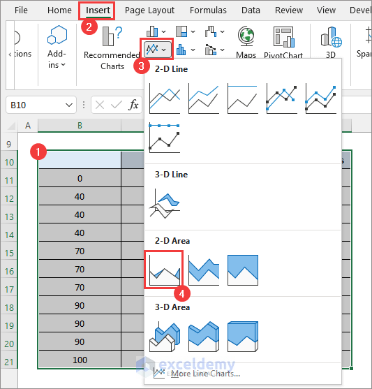
Step 4: Insert Area Chart

After that, select the entire table and go to Insert >> Insert Line or Area Chart >> 2-D Area >> Area.

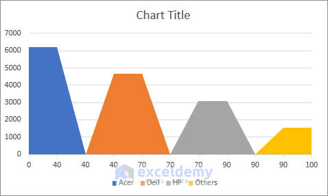
Then you will get the following chart. Rename the Chart Title as required by clicking on it.

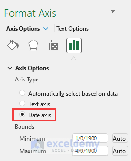
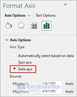
Next, right-click on the horizontal axis and select the Format Axis.

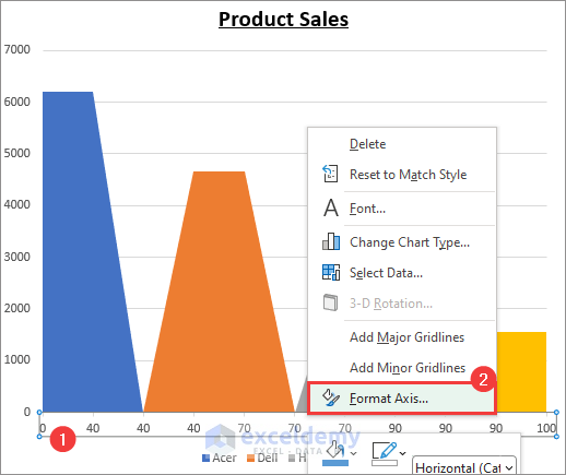
Then change the Axis Type to Date Axis. Next, enable Data Labels and apply any other formatting as required.

Finally, you will get the following column chart with varying widths.

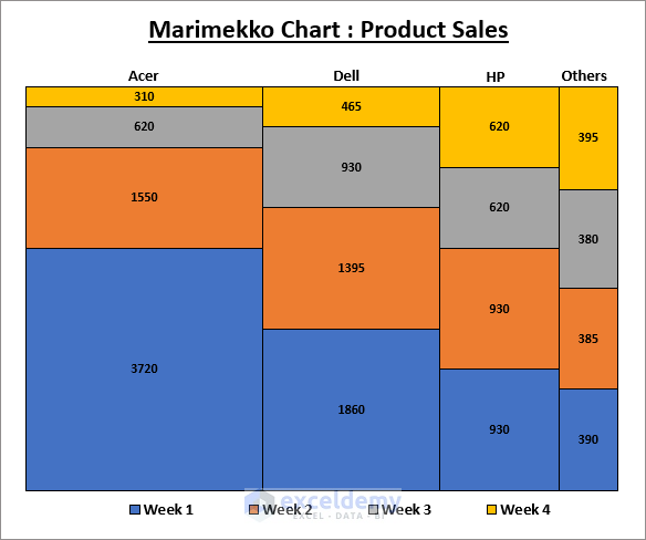
How to Create a Marimekko (Mekko) Chart in Excel

Suppose you have the following dataset showing the weekly sales instead of the total month. Now you want to create a Marimekko (Mekko) chart with this data.

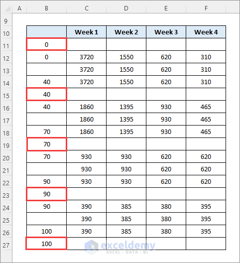
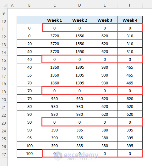
First, create a duplicate table from the original dataset as follows. It contains the cumulative sales percentages of the sales amounts as in the earlier method. But this time copy the sales three times instead of two and keep a blank row between sales for each brand as earlier.

Then, type 0 and 100 in the first and last cells of the first column (not labeled) respectively. Next, fill the blank cells with the same value of the adjacent cells above and below if those values are the same too. For, example type 40 in cell B15 as both B14 and B16 contain 40.

Next, fill the remaining blank cells in this column with the average of the values of the adjacent cells above and below. For example, enter (40+70)/2= 55 in cell B17.

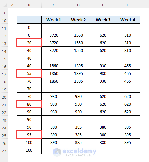
After that, fill the blank rows with 0 as shown below.

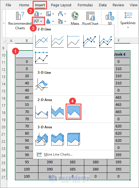
Now select the entire table and go to Insert >> Insert Line or Area Chart >> 2-D Line >> 100% Stacked Area.

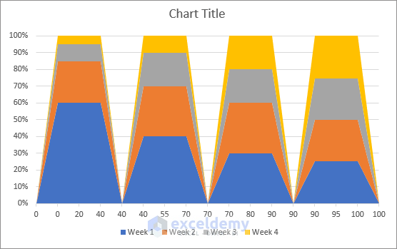
Then you will get the following chart. Change the Chart Title as required.

Now right-click on the horizontal axis and select the Format Axis.

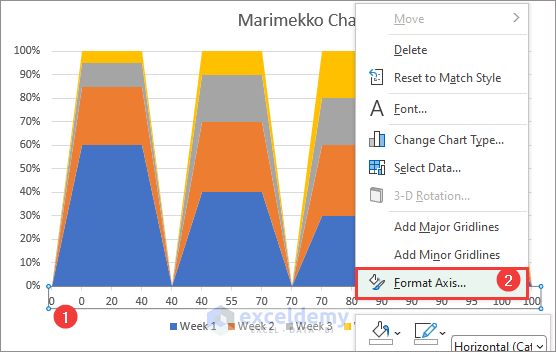
Then change the Axis Type to Date Axis as earlier. Next, enable Data Labels and apply Outline to each data Series.

Finally, you will get the marimekko chart as follows.

Things to Remember

Make sure the percentage values are not fractions but rather whole numbers.
You need to manually delete the unnecessary data labels. As there are many zeros in the data table, data labels will also be stacked upon one another. Keep deleting until all of them get deleted.

Download Practice Workbook

You can download the practice workbook from the download button below.

Variable Width Column Chart.xlsx

Conclusion

Now you know how to create a variable width column chart and a marimekko (Mekko) chart in Excel. Do you have any further queries or suggestions? Please let us know in the comment section below.

<< Go Back To Column Chart in Excel | Excel Charts | Learn Excel

Get FREE Advanced Excel Exercises with Solutions!