Suppose you own a restaurant and want to know about your shop’s best-selling product. You can calculate the profit, sorting the number to see which one is higher, or you can use Treemap to spot patterns, such as which items are the restaurant’s best sellers. This article will teach us how to make a Treemap chart in Excel.
What Is a Treemap Chart in Excel?
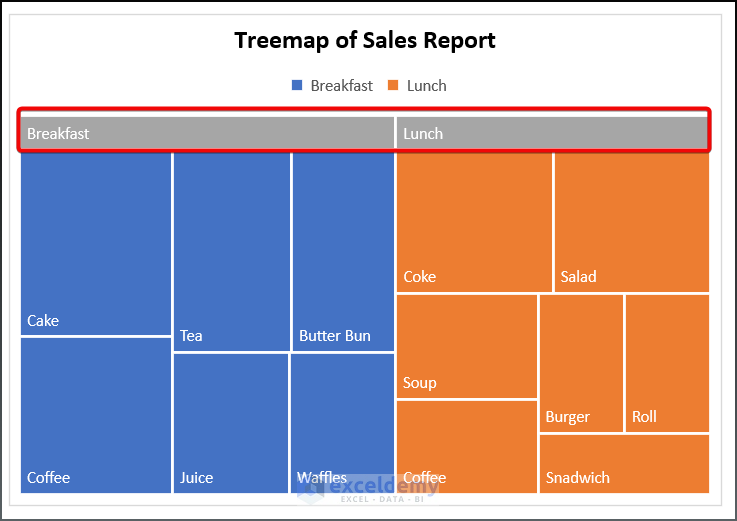
An Excel Treemap chart creates a chronological order to provide a better understanding of your dataset. In this type of diagram, the tree branches are shown as rectangular boxes, and each branch’s sub-branch is shown as a smaller rectangle.
A typical Treemap chart can be depicted as follows:
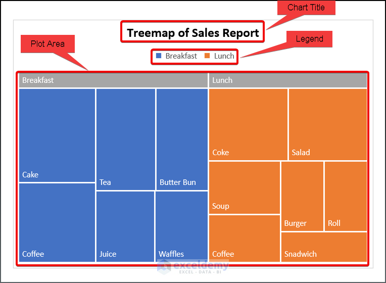
As the figure shows, a Treemap chart mainly consists of 3 sections:
- Chart Title: The chart’s heading, gives your chart a descriptive name to understand the visualization more easily.
- Legend: The legend serves as a map to identify various data series.
- Plot Area: The visual representation happens in this area. The top-level categories are used to color each rectangle, and each item’s subcategory (or sub-branch) rectangle is drawn according to the magnitude of the numerical value it contributes to the overall dataset.
How to Make a Treemap in Excel: 2 Easy Methods
Let’s assume we have a dataset, namely “Sales Report of the Restaurant”. You can use any dataset suitable for you.
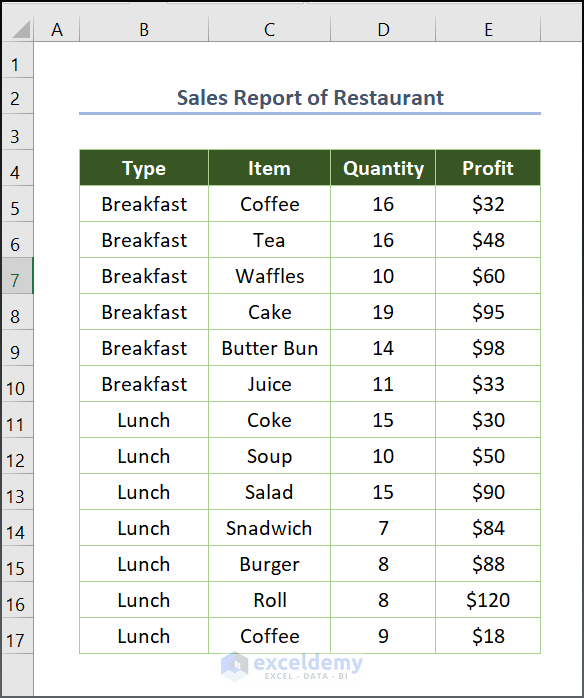
Here, we have used the Microsoft Excel 365 version; you may use any other version according to your convenience.
1. Creating a Treemap from the Charts Ribbon Group
There are several ways to create a Treemap using the built-in Treemap command. There is no hard and fast rule to use one in a particular way. All processes will yield the same output. However, we have discussed two ways to do so, and later, we will customize our chart.
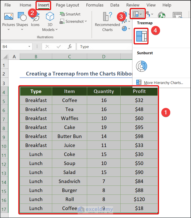
📌 Step 1: Pick Treemap Chart on the Insert Tab
- First, open your Microsoft Excel and select the data. To select your data, drag your cursor from the top left corner to the bottom right corner of the data by simultaneously holding the mouse’s left button.
- Click on the Insert button in the Menu Bar.
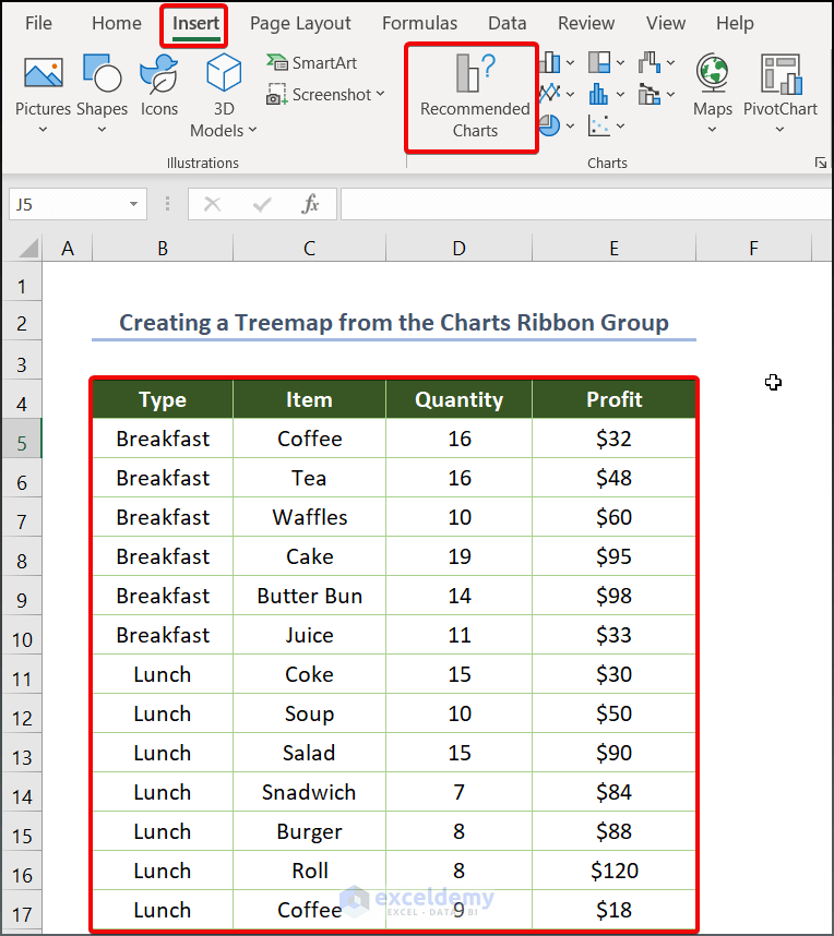
Alternatively, you can create a Treemap chart by clicking on the Recommended Charts command on the Insert tab. Also, you can click on the dialog launcher located at the lower-right part of the Charts ribbon group.
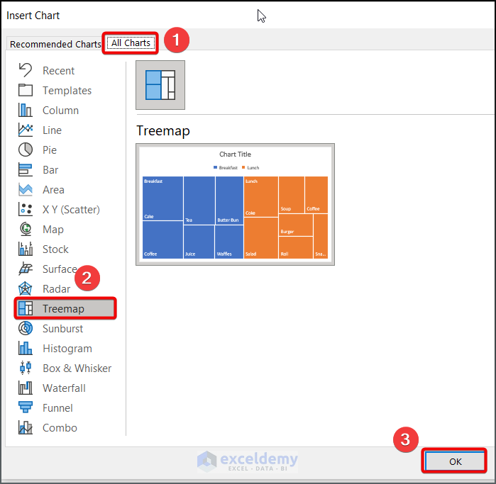
- Subsequently, select All Charts>> Treemap>> Press OK to generate a Treemap chart.
- The action you have taken will bring a Treemap chart like the one below:
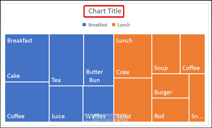
- Change the Chart Title by simply double-clicking on it. Then give an entry of your desired title.

For each of the top-level or parent categories, Excel automatically selects a different color. To differentiate between the categories, you can also use the layout of the data labels.
📌 Step 2: Format the Data Label Options
If you wish, you can format the data labels in Excel Treemap based on your requirements.
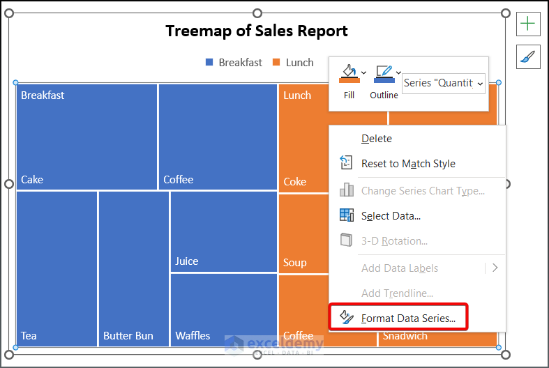
- To change the label display, right-click one of the rectangles on the chart, then click on Format Data Series…
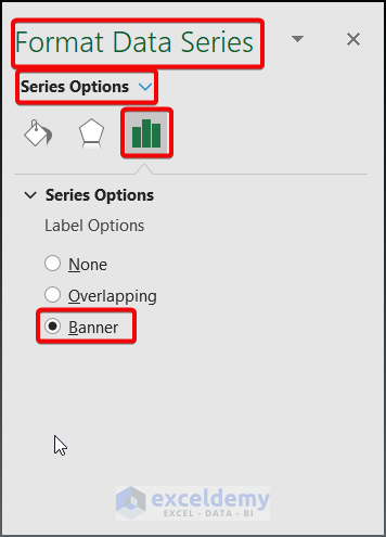
- This will bring an interface like below. Under Series Options, select Banner to get label data on top of the chart area.
- This action will allow you to have labeled data as shown below:
📌 Step 3: Change Chart Layout and Styles
When it relates to describing your chart, preset layouts are always a smart place to start. The Chart Design tab provides styling options.
- Click on the Treemap chart to appear a Ribbon like the following one.
- Then select the Chart Design option to have some preset layout like below.
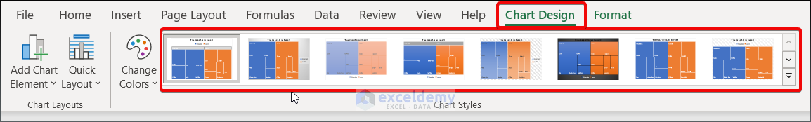
- Choose your chart style at your convenience. I have selected one that yields output like below.

📌 Step 4: Change Chart Colors
- This is also a similar process as we did while changing our layout. Click on the chart first, select Chart Design, and then move on to the Change Colors option, where you can find many opportunities to change your chart area’s color.
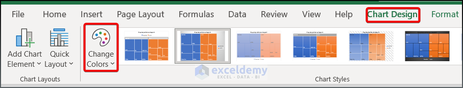
- I have selected one to show you the output. You can choose whatever seems good to you.

📌 Step 5: Resize Treemap Chart
You can move and resize your chart to any desired spot on your existing spreadsheet using Microsoft Excel. Select your chart, then drag and drop it to the desired location on your worksheet. To resize the chart, drag it from a corner or edge inward or outward. If you want to make your chart smaller, drag it toward the center; if you want to make it larger, drag it away from the center.

So, you can create the Treemap chart in Excel utilizing these five steps.
Read More: Create Treemap Chart to Show Values in Excel
2. Using SmartArt Graphic Tool
In this section, we will talk about how you can create a Treemap by using the SmartArt Graphic tool. Basically, this is a manual method and quite handy if you’re accustomed to using the SmartArt tool. Before diving into the process, let me know you all, this is a manual process, which I found tiresome to some extent.
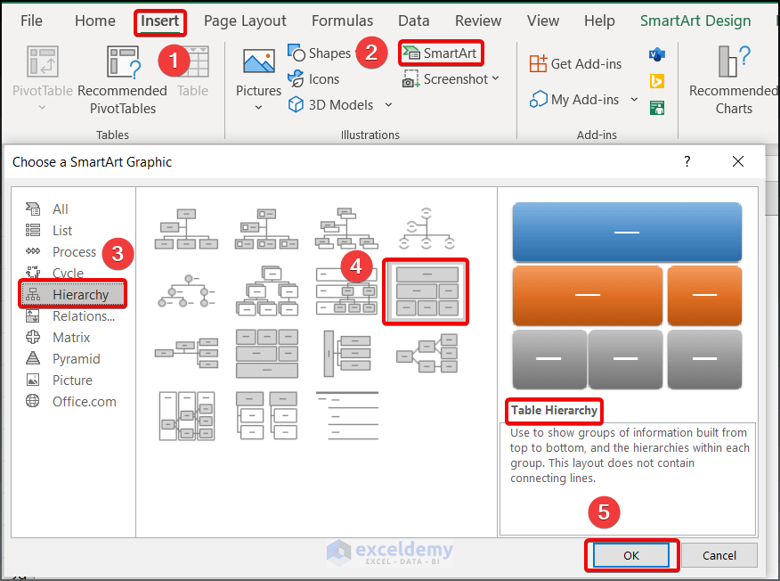
- First, click on the Insert tab, and select the SmartArt tool. This will bring a dialogue box, and then select Hierarchy>>Table Hierarchy>>OK.
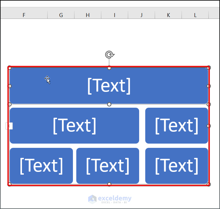
- Thus, the following shapes will appear.
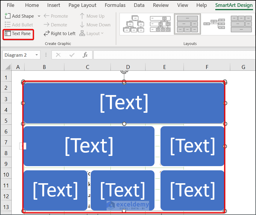
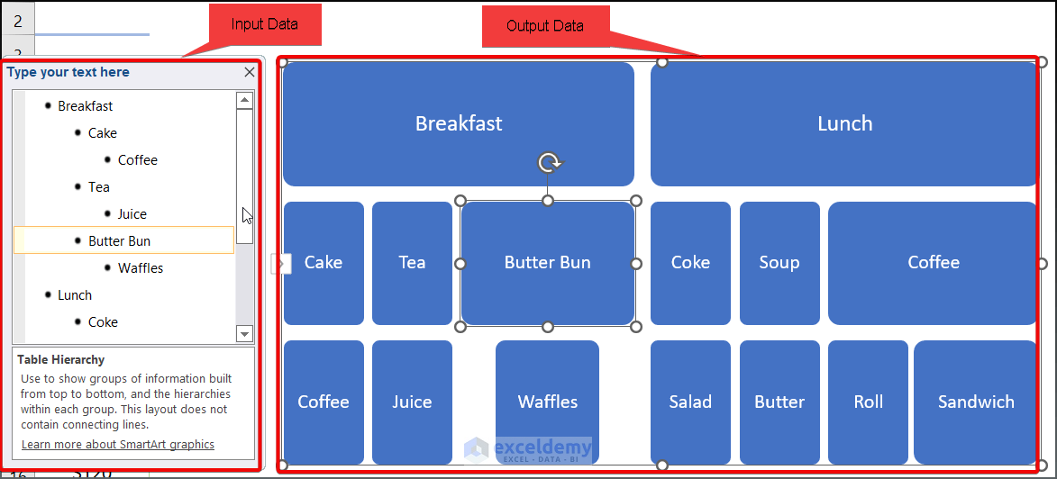
- To input your data, double-click on the rectangular box, then select Text Pane
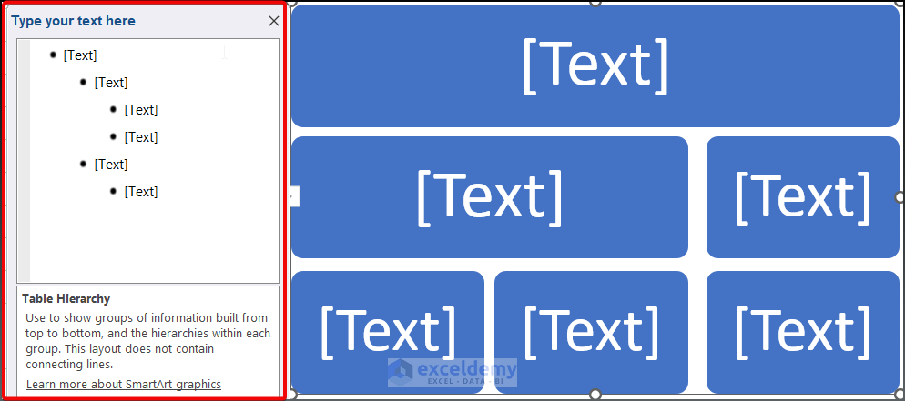
- Then you will enter your data by following the hierarchy.
- Here, I have provided the input and output data for our better understanding.
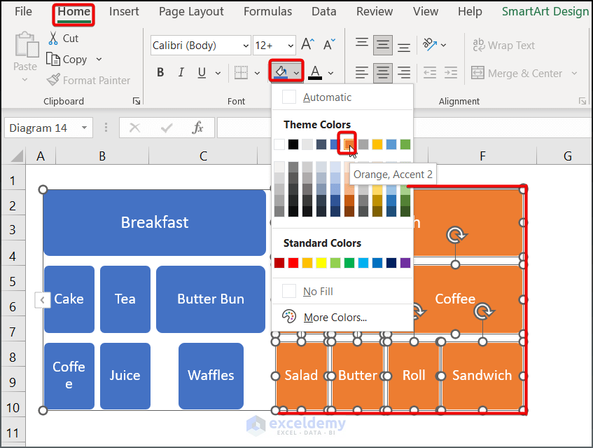
- Now, you can mark the blocks by changing their color. To do so, select the intended block by holding the CTRL button on your keyboard and label the block by your preference.
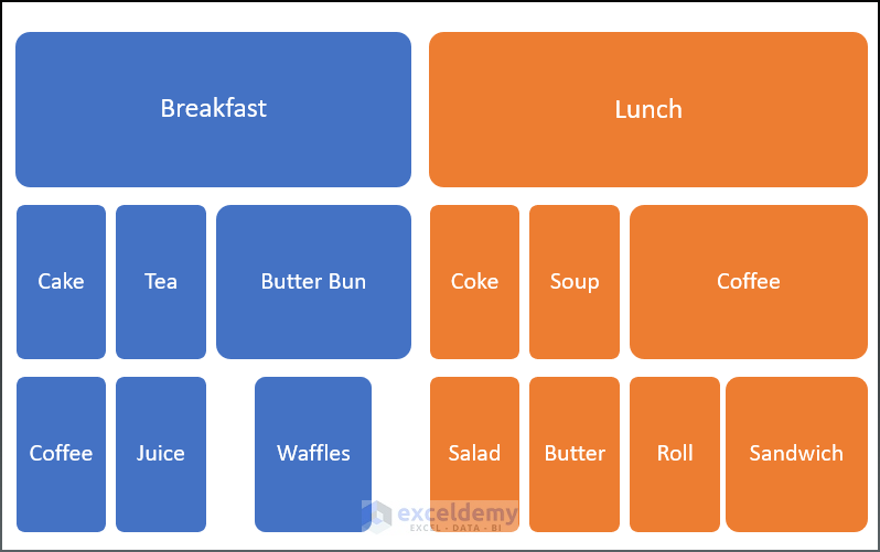
After changing the color, you’ll get the following output, the same as the first method.
Read More: How to Create Hierarchy Tree from Data in Excel
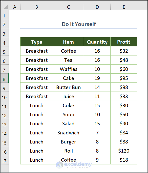
Practice Section
We have provided a practice section on the right side of each sheet so you can practice yourself. Please make sure to do it yourself.
Download Practice Workbook
You can download and practice the dataset that we have used to prepare this article.
Conclusion
Hopefully, you all have had hands-on experience with how to make a Treemap in Excel. Feel free to comment below if you have any queries regarding this lesson. Thank you!
Related Article
<< Go Back to Treemap Chart Excel | Excel Charts | Learn Excel
Get FREE Advanced Excel Exercises with Solutions!
