How to Add and Format Data Labels in an Excel Treemap

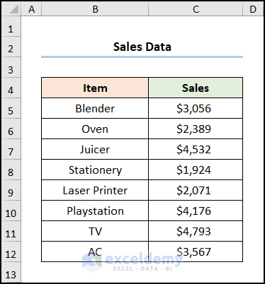
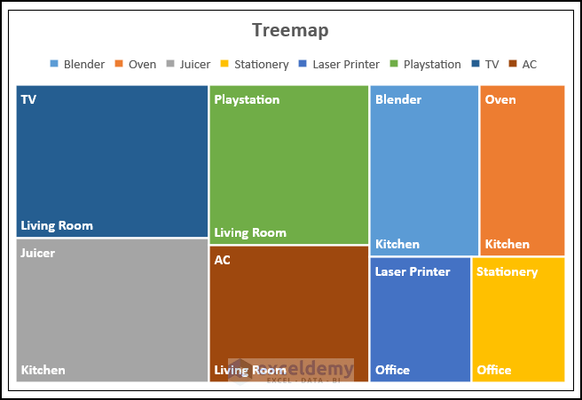
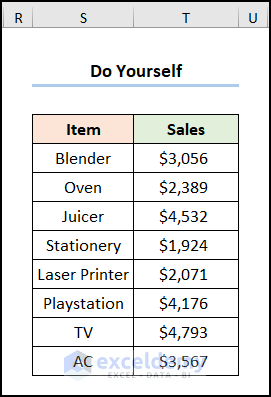
Consider the Sales Dataset containing Items and Sales in USD.

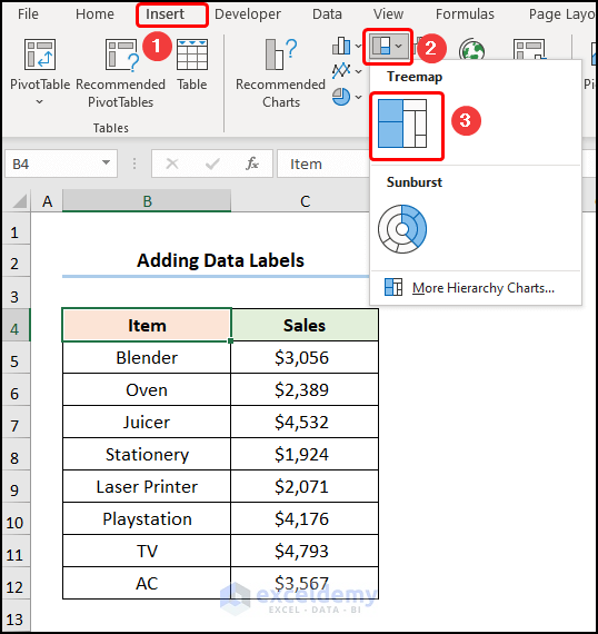
Step 1 – Insert a Treemap chart

• Go to the Insert tab >> click Insert Hierarchy Chart >> choose Treemap chart.

Read More: How to Create Hierarchy Tree from Data in Excel

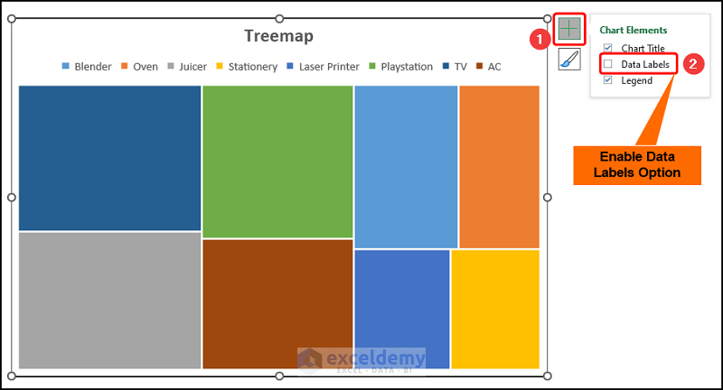
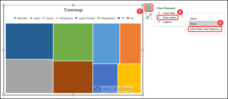
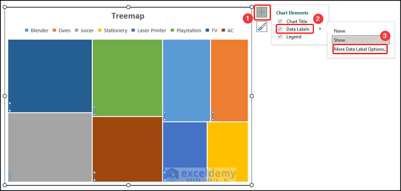
 Step 2 – Add Data Labels

• Click Chart Elements >> Check Data Labels.

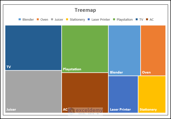
Data labels are added.

5 Ways to Format Data Labels in an Excel Treemap

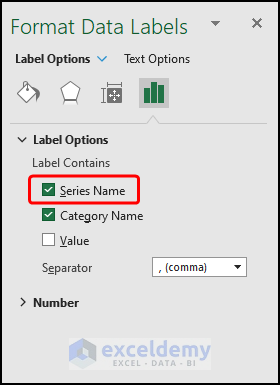
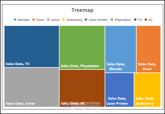
1. Series Name

• Select the chart >> click Chart Elements >> In Data Labels, choose More Data Label Options.

• In Format Data Labels, check Series Name.

This is the output.

2.  Category Name

• Select the chart >> click Chart Elements >> In Data Labels, choose More Data Label Options.

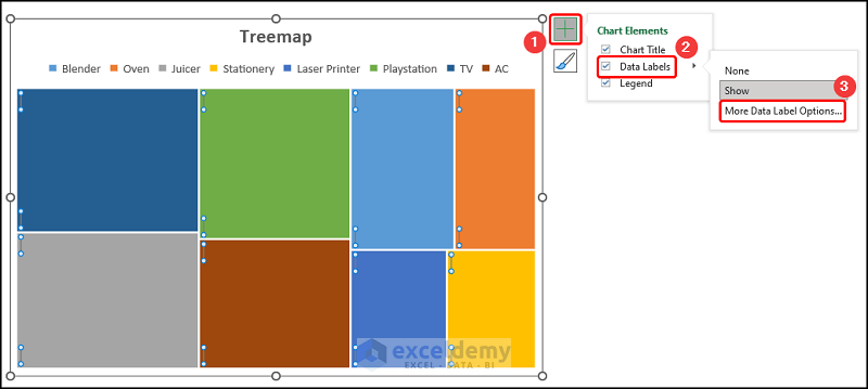
• In Format Data Labels, check Category Name.

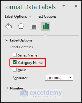
This is the output.

3. Showing Values in the Chart

• Go to More Data Labels Options by following the steps described previously.

• In Format Data Labels, check Value.

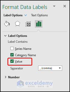
This is the output.

Read More: Create Treemap Chart to Show Values in Excel

4. Number Option

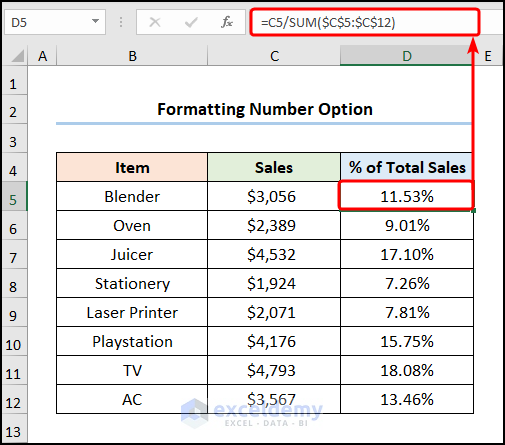
• Go to D5>> enter the following expression into the Formula Bar >> use the Fill Handle tool to copy the formula into the cells below.

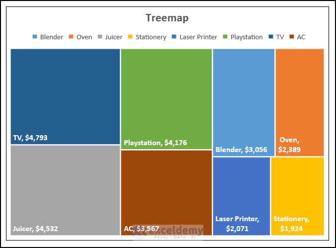
C5 cell refers to  “Blender Sales of $3,056”, whereas C5:C12 represents the “Sales” column.

Note: Use an Absolute Cell Reference by pressing F4 and change the cell formatting to percentage by pressing CTRL + SHIFT + 5.

• Go to the Insert tab >> choose Treemap.

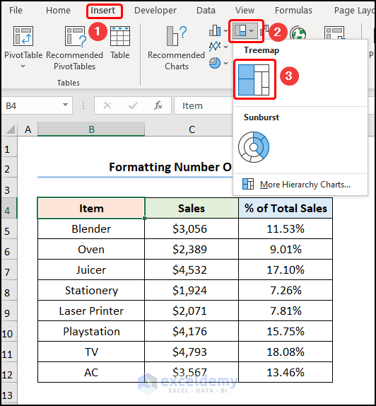
• In Chart Elements, select More Data Labels Options.

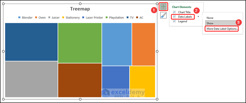
• Check Category Name and Value >> choose Percentage.

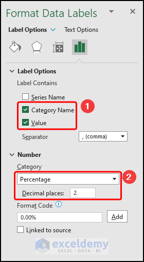
This is the output.

Read More: How to Change Treemap Order in Excel

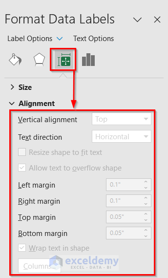
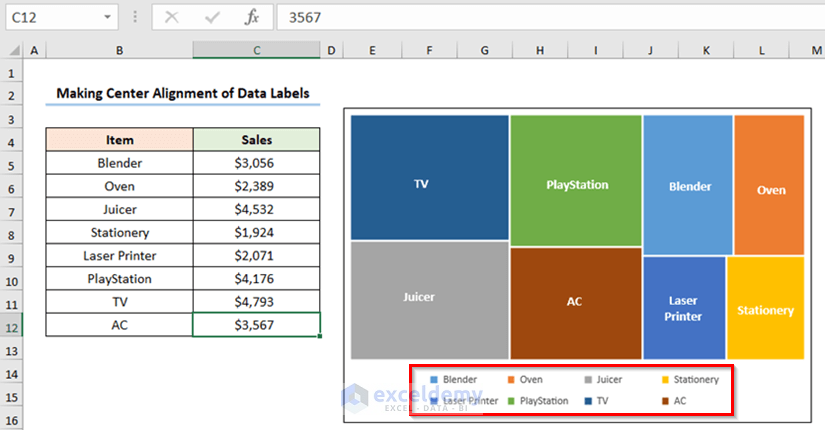
5. Changing the Alignment

By default, data labels will be on the left side of the chart. You can manually change this format.

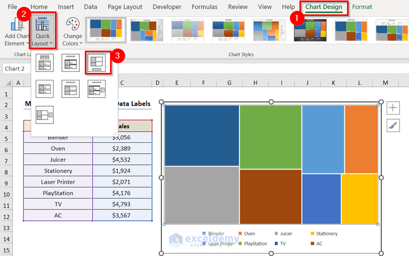
• Select the chart >> Chart Design >>Quick Layout >> Layout 3 [Shows the following chart element – Legend (bottom)].

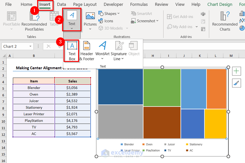
• In the Insert tab >> go to Text >> choose Text Box >> drag the box onto the chart.

• Select the box >> Shape Format >>  Shape Fill >> No Fill >> Shape Outline >> No Outline.

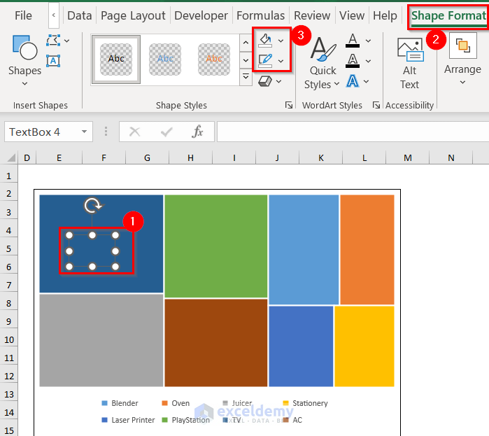
• Enter the data label: TV.
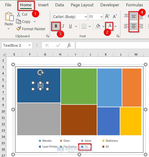
• Select that text >> Home tab >> change the Font color >> make it Bold >> make the alignment Middle and Center.

• Copy the 1st Text Box by pressing CTRL+C >> paste it by pressing CTRL+V
• Enter data labels for each portion of the chart.
• Select all text boxes >> right-click  >> Group them.
• If you move the chart, text boxes will also move.

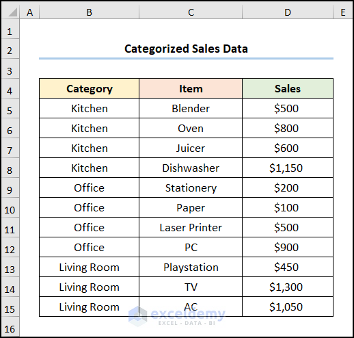
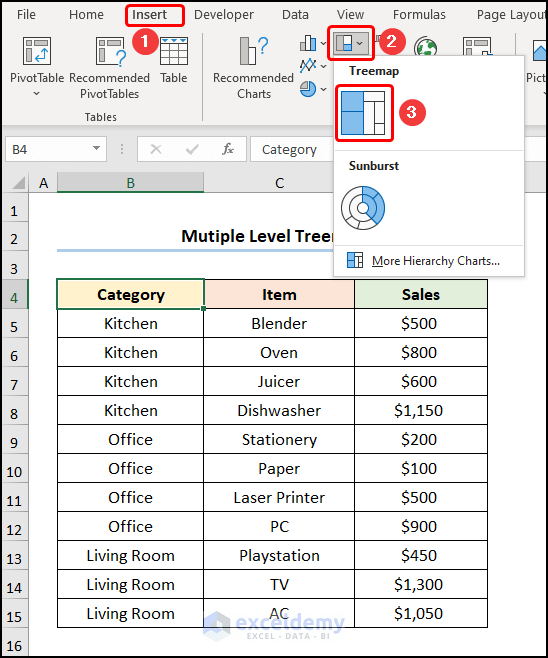
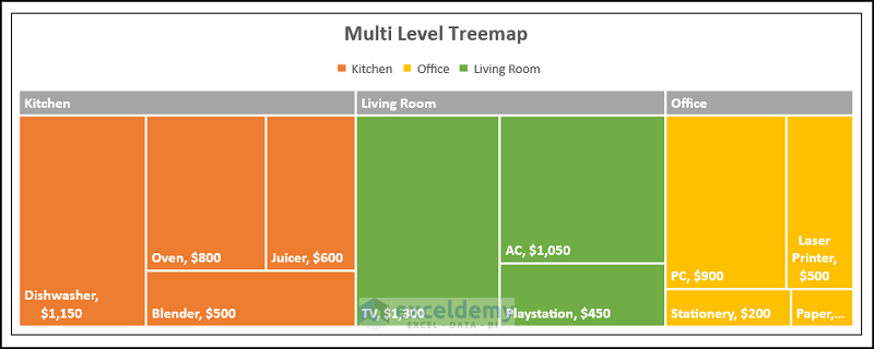
How to Add Multiple Levels in to an Excel Treemap

The dataset showcases Categorized Sales Data with Category, Item, and Sales in USD.

Steps:

• Go to the Insert tab >> Select Treemap.

• Select Chart Elements >> go to More Data Labels Options.

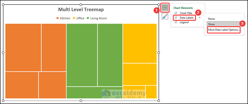
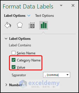
• Check Category Name and Value.

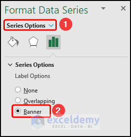
• In Series Options >> select Banner.

This is the output.

Practice Section

Practice here.

Download Practice Workbook

<< Go Back to Treemap Chart Excel | Excel Charts | Learn Excel