Significant numbers are significant because they enable us to monitor the accuracy of measurements. In essence, sig figs show how much to round while simultaneously ensuring that the result is not more accurate than our initial value. This article will show you how to keep significant figures in Excel.
How to Keep Significant Figures in Excel: Step-by-Step Procedures
In the following steps, we will demonstrate to you how to keep significant figures in Excel by applying the ROUND function with the combination of the INT function, the LOG10 function, and the ABS function. And we will also show the change of significant figures on the Excel graph axis.
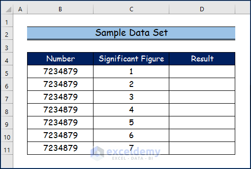
Step 1: Creating Data Set
- Firstly, we will create our data set to keep the 6 significant figures in Excel.
Step 2: Applying ROUND Function
- Firstly, select the D5 cell.
- Then write down the following formula.
=ROUND(B5,C5-(1+INT((LOG10(ABS(B5)))))Formula Breakdown
- First, it’s always useful to start from the outside when you have a formula like this where one function (in this instance, ROUND) loops around all the others. Therefore, this formula’s fundamental step is utilizing the ROUND function to round the number in the B5 cell.
=ROUND(B5, X)
- Here x is the necessary number of significant digits. Calculating X in this formula is difficult. Given that it will vary based on how the number is rounded, this is a variable. This bit is utilized to calculate X.
C5-(1+INT((LOG10(ABS(B5))))
- The ABS function returns the positive value, and it returns 7234879.
ABS(B5)
- LOG10(ABS(B5)): This portion of the formula gives the value, which is 6.859.
=LOG10(ABS(B5))
- INT((LOG10(ABS(B5))): This portion of the formula returns the lowerest integer which is 6 in this case.
INT((LOG10(ABS(B5)))
- C5-(1+INT((LOG10(ABS(B5)))): Here the value of the C5 cell is So, C5-(1+INT((LOG10(ABS(B5)))) = 1-(1+6 )=-6. It displays the number’s remaining digits, excluding the first six.
C5-(1+INT((LOG10(ABS(B5))))
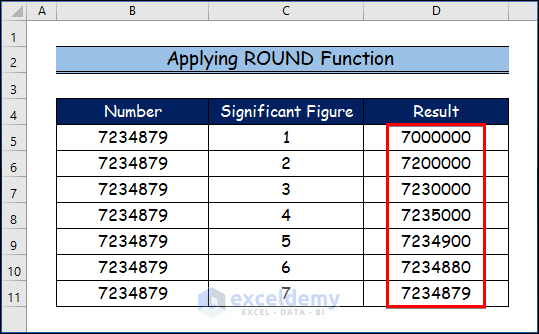
- =ROUND(B5,C5-(1+INT((LOG10(ABS(B5))))): This final formula represents the first significant value, which is 7000000.
=ROUND(B5,C5-(1+INT((LOG10(ABS(B5)))))
- Now, press ENTER.

- Therefore, you will observe the result for the first significant figure in the D5 cell in the below image.
- Then, use the Fill Handle tool and drag it down from the D5 cell to the D11 cell.

Step 3: Showing Final Result
- Finally, here is our final outcome for all the six significant figures in the D column.
Read More: How to Change Significant Figures in Excel
Changing Significant Figures in Excel Graph Axis
Typically, an Excel graph is intended to establish a trend and help readers better grasp the data. You might have changed a graph’s legend and added axis titles. However, there are situations when you might need to update important numbers in an Excel graph. In this section, you will learn how to change significant figures in an Excel graph.
Step 1: Utilizing Charts Group
Excel’s charts group provides a range of chart types. In particular, many charting tools enable users to visualize complex data in straightforward, graphical forms.
- Firstly, go to the Insert tab after selecting the data range from the given data set.
- Secondly, choose the Insert Column or Bar Chart from the Charts group.
- Thirdly, select the Clustered Column option from the 2-D Column.

Step 2: Creating Column Chart
Here, we have created a column chart based on our data set which has decimal points, but we have not shown decimal points.
- So, you will see the column graph between product name and price without a decimal point.

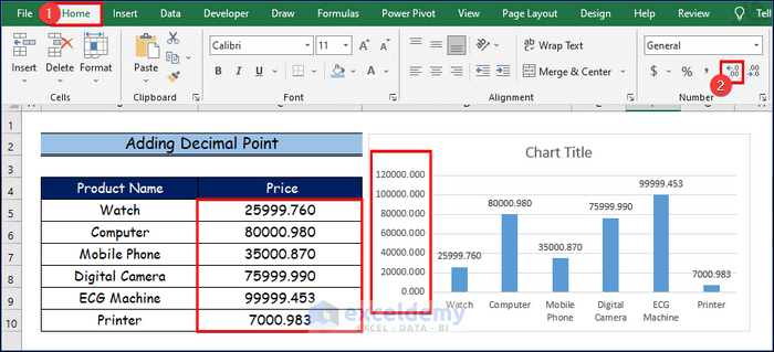
Step 3: Adding Decimal Point
In this section, we will change the significant figure in our data set by adding a decimal point in the price column.
- Here, select the Price column.
- Then, go to the Home tab.
- After that, click on the icon at position 2 which indicates the increase of decimal points.
- Finally, you will notice that the axis label has changed to decimal points with the price column here in the data set.
Download Practice Workbook
You may download the following Excel workbook for better understanding and practice it by yourself.
Conclusion
In this article, we’ve covered step-by-step procedures to keep significant figures in Excel. We sincerely hope you enjoyed and learned a lot from this article. If you have any questions, comments, or recommendations, kindly leave them in the comment section below.
Related Articles
<< Go Back to Significant Figures | Rounding in Excel | Number Format | Learn Excel
Get FREE Advanced Excel Exercises with Solutions!
