How to Change Significant Figures in Excel (2 Easy Methods)

Nowadays displaying numbers, with a certain number of significant figures, is very essential not only in the scientific community but also in other fields. But unfortunately, Excel doesn’t have any single built-in formula to display or change significant figures. Hence, to change a significant figure, one has to use a custom formula. In this article, we will show you 2 easy and efficient methods to change significant figures in Excel.

How to Change Significant Figures in Excel: 2 Useful Methods

In this section, we will demonstrate 2 effective methods to change significant figures in Excel with appropriate illustrations.

1. Combine ROUND, INT, and ABS Functions to Change Significant Figures

You can easily use the formula below to change significant figures in a given number. The syntax of our formula is,

=ROUND(Number,SF-(1+INT(LOG10(ABS(Number))))

The formula is a bit complex. But we will walk you through the formula and explore it step by step. Let’s start!

Step 1:

First of all, let’s get familiar with the 4 functions used in this formula

1. 1. The ROUND function.
   2. The INT function.
   3. The LOG10 function.
   4. The ABS Function.

ROUND Function:

• This function has 2 arguments.

=ROUND(number, num_digits)

• In the 1st argument, you have to insert the number you want to round.
• In the 2nd argument, put the decimal place up to which you want to round.
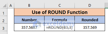
• Let’s take an example. Suppose you want to round 357.5687 up to 3 decimal places. You have to insert the formula.

• And the result will be 357.569

• But if you want to round it by the nearest hundreds, you have to input -2 in the 2nd argument ( Because the hundreds place is 2 steps left from the decimal place). Like this:

The result will be 400.

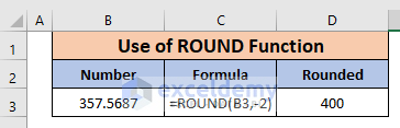
• Look at the value carefully. It contains only 1 Significant Figure (SF).
• Let’s take another value such as 7856.964. Now if we want to express the value with only 1 SF, the 2nd argument in the formula should be -3.

• Hence, it is clear that we can express any value to any significant figure with the ROUND But we have to manually calculate the value of the 2nd argument for different numbers. It depends on how many numbers are there on the left or right side of the decimal place.
• To get rid of this problem, and make the process automatic, we use the functions below.

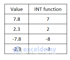
INT Function:

• It rounds a number down to the nearest integer. Some examples are given here.

LOG10 Function:

• This function returns the base-10 logarithm of a number. Examples are shown below.

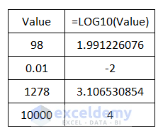
• Note that here the argument must be a positive value. Hence we have to make the argument positive.

ABS function:

• It returns the absolute value of a number.

Step 2:

• Now that we have got familiar with our functions, let’s see how the formula as a whole work.

Here the number 78364556.96 will be rounded to 1 SF.

• In the Abs Value column, apply the ABS

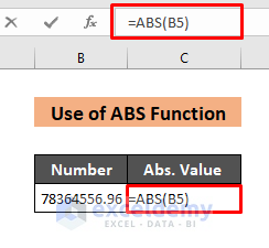
• Returns the absolute value of 78364556.96

• In the Log of Abs Value column, we will use the LOG10 funtion.

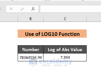
• Which gives the base 10 logarithm which is 7.894
• In the Rounding to Nearest Integer column, the formula is,

• That round downs the number to its closest integer 7.

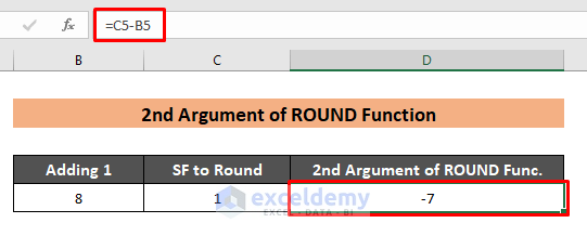
• In the Adding 1 column, the formula used is

• This gives the value of 8

• In the 2nd Argument of Round Func. column, we use the following formula,

• This gives the value up to which the number should be rounded which is -7.

Step 3:

• In the Final Result column, we used the ROUND function to get the final result. The formula is,

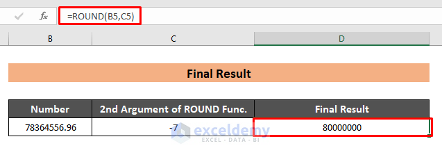
• which gives our desired value which is 80000000.
• So the formula of the whole process is,

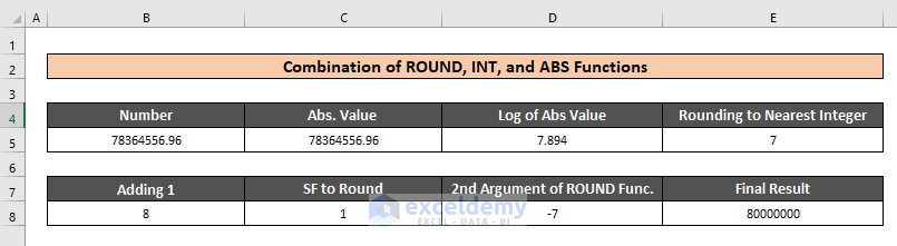
• Similarly, the number is rounded up to 6 SF using the same formula below:

Read More: How to Change Significant Figures in a Graph in Excel

2. Apply a User-Defined Function to Change Significant Figures

You can create a custom function by using VBA code to do the same task of changing the significant figure in Excel. Follow the steps below.

Steps:

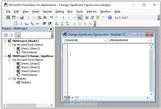
• Press Alt+F11 to open the ‘Microsoft Visual Basic for Applications’ You can also do that by going to the Developer ribbon and selecting the Visual Basic option.

• You will see a window like this.

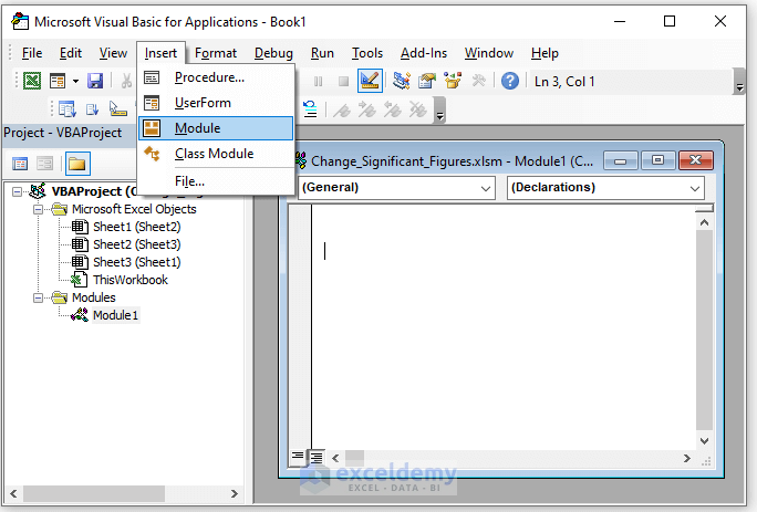
• Now go to the top menu bar and click on Insert, you will see a menu like this. From the menu, select the “Module”

• Here, a new “Module” will appear. Now paste the following VBA code into the box.

Function SigFig(Value As Variant, Digits As Variant)
Dim exp As Double
If IsNumeric(Value) And IsNumeric(Digits) Then
If Digits < 1 Then
' Please Insert the  " #NUM "  error
SigFig = CVErr(xlErrNum)
Else
If Value <> 0 Then
exp = Int(Log(Abs(Value)) / Log(10#))
Else
exp = 0
End If
SigFig = WorksheetFunction.Round(Value, _
Digits - (1 + exp))
End If
Else
' Please Insert the  " #N/A "  error
SigFig = CVErr(xlErrNA)
End If
End Function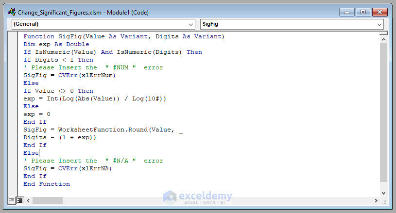

• After pasting the code, go back to the worksheet. Now you can use the function SigFig.

Where,

• In the first argument, you have to input the number.
• in the 2nd argument input the SF.

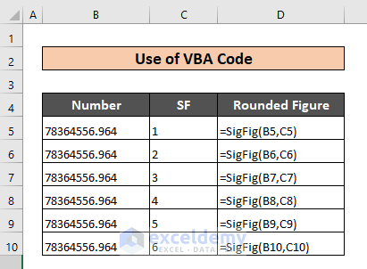
• Press ENTER to see the result. The result will be the same as the previous method.

Similar Readings:

• How to Count Significant Figures in Excel
• How to Keep Significant Figures in Excel

Things to Remember

• In the 2nd method, you must insert a new Module to paste the VBA code, otherwise, the user-defined function will not be available in Excel.
• In the 1st method, you can use the LOG function instead of LOG10. But you must ensure that the 2nd argument is not other than 10.

Download Practice Workbook

Download this practice workbook to exercise while you are reading this article.

Conclusion

By using the above methods, you can change the number of significant figures in Excel as per your wish. Hence it will give you the power to take the command from Excel to yourself on how your data will be displayed and how many significant figures they will contain. If you find this article helpful, please share this with your friends and don’t forget to share your feedback in the comments section.