How to Create a Recipe Database in Excel (2 Easy Steps)

The article will show you how to create a recipe database in Excel. It is one of the real-life applications of Excel. We eat different types of food in our meals. But sometimes we like to taste foods of special categories which are made following some special processes. We can get the idea of making them by searching on the internet, but storing the processes in Excel will help us to find them easily if we want to cook those special foods in the future.

Watch Video – Create a Recipe Database in Excel

How to Create a Recipe Database in Excel: 2 Easy Steps

In the following picture, I’ve given a preview of how a recipe database may look like. You can make it look stylish, and format some cells that contain special recipes, but to make the topic easily understandable, I’m keeping it simple. I’ll also use some functions and commands so that you can find a recipe instantly if your dataset contains a lot of recipes.

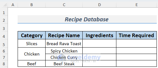
Step-1: Inserting Necessary Columns for Recipe Database

The first thing you should do while creating a database is to add some columns that will contain vital information about a recipe. Let’s have a look at the description below.

First, select some cells to store the recipe information and type the heading. Also, you may choose the category and food item that you want to make in the future.

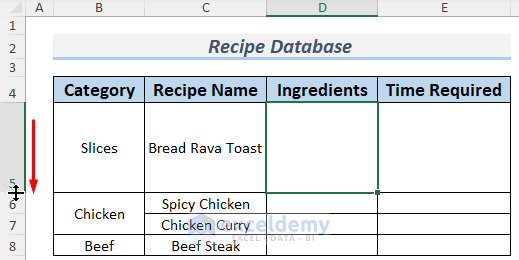
Next, we will insert the corresponding ingredients. But as you have seen, we filled all the ingredients for a recipe in a single cell. For that purpose, we need to increase the row height. Just put the cursor in the place shown in the following image and drag it below.

After that, start typing the ingredients. When you finish typing the first ingredient, then press ALT+ENTER. This will take your cursor to the next paragraph.

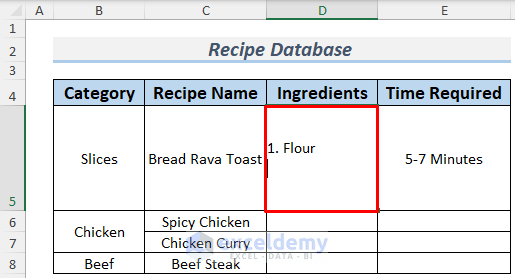
Similarly, type all the other ingredients for that recipe and press the ENTER.

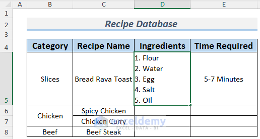
Thus you can fill all the ingredients in one cell for each recipe. Basically, your recipe database is created after this.

Step-2: Filtering Recipes from the Recipe Database

Now we will create some features with Excel functions and commands so that you can use the recipe database effectively. Please follow the instructions below.

1. Filtering by IF Function and Data Validation

We can use the IFS (family function of IF) and INDIRECT functions to apply some filters to the recipe database. Please go through the following section to get a better understanding

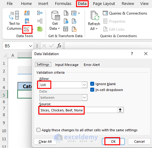
First, open a new sheet and select a cell to store the Data Validation.
Next, go to Data >> Data Validation (from the Data Tools group).
In the Data Validation window, select List from the Allow section and type the Category names in the Source.
After that, click OK.

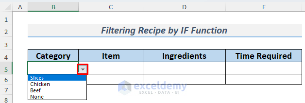
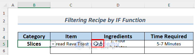
Thereafter, you will see the Data Validation list in B5. Click the drop-down icon to see this.

Next, we are going to use the following formula to get the recipe overview when we select a category from the Data Validation

=IFS(B5="None","",B5='recipe list'!B5,INDIRECT("'recipe list'!C5:E5"),B5='recipe list'!B6,INDIRECT("'recipe list'!C6:E7"),B5='recipe list'!B8,INDIRECT("'recipe list'!C8:E8"))

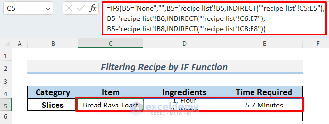
Here, the formula uses the IFS and INDIRECT functions. The formula looks a bit complex but in reality, it just contains some conditions and arrays. We are checking whether the category in B5 matches the category in the recipe list sheet (please download the file for a better understanding). It then returns corresponding recipe items, ingredients, etc.

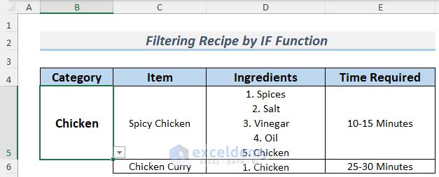
If you look at the image above, you can see that the cell containing the ingredients is not clear. For that reason, we will use the Format Painter to format this cell properly.
Go back to the Recipe Database sheet and select one or multiple cells (Here I selected D6:D7.
After that, select Home >> Clipboard >> Format Painter.

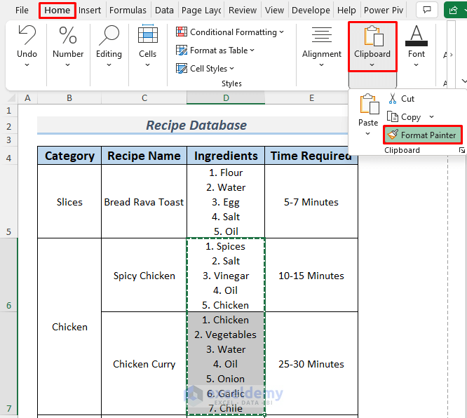
Later, go to the Filtering sheet and place the Format Painter icon on the cell that you want to format. Just click on it.

This operation will make the cell format of D5 of the Filtering sheet similar to the previously selected cell. Let’s select another category from the Data Validation List and see how it goes. The Chicken Category has two items, so two items will show up.

The second item’s ingredients are not visible now. So to view them, just increase the row height by double-clicking on the mouse when you put the cursor on the corresponding row and the following icon appears.

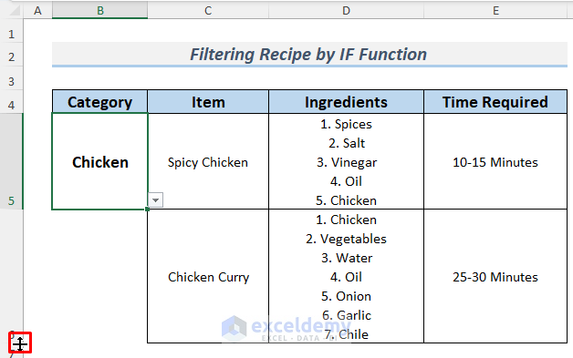
Thus, you can filter the recipe item so that you can find your desired one easily from a large recipe database.

2. Filtering by Filter Command

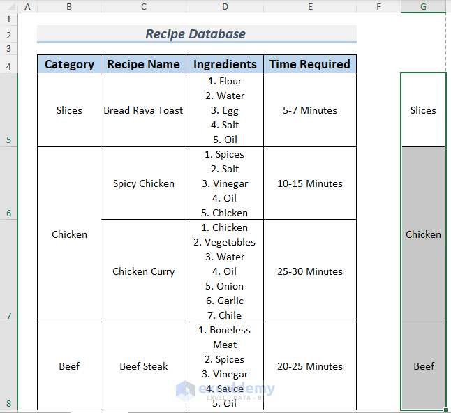
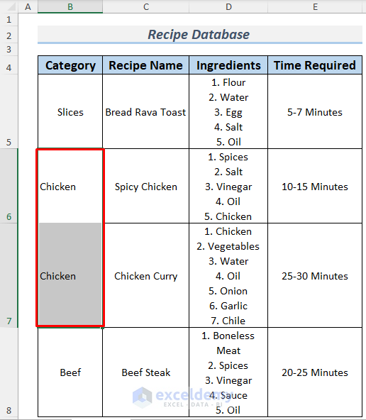
We can also filter the recipe items by using the Filter command. This is an easy process but it needs some tricks to apply.

Notice that the Category Chicken is merged through B6:B7. If we apply Filter to this data, some of the data will not appear.
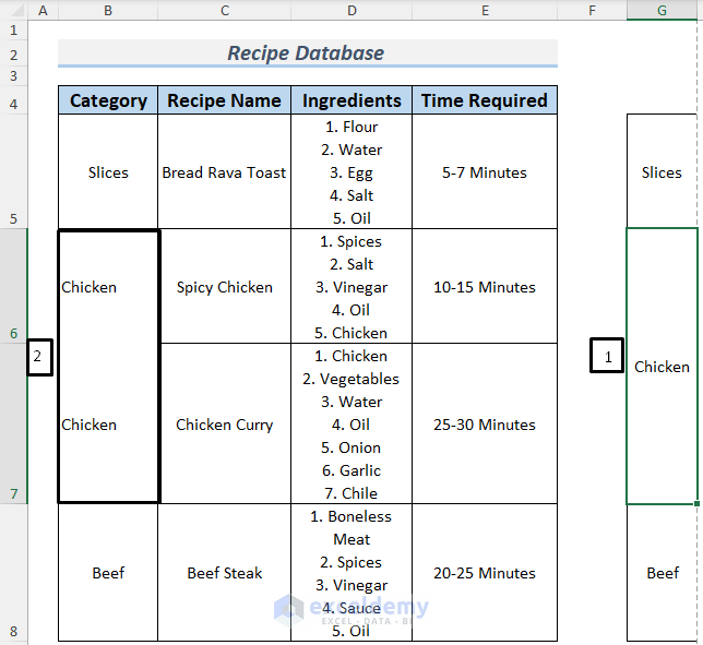
So, first, copy the cells B5:B8 and paste them somewhere in the sheet. Here I pasted them in G5:G8. G6:G7 will remain a merged cell.

After that, unmerge the cells (B6:B7). You can find this option in the Alignment group of the Home Tab.

Thereafter, simply use the Format Painter to copy the format of G6:G7 merged cells and paste it to B5. The process of using the Format Painter is described in the previous process.

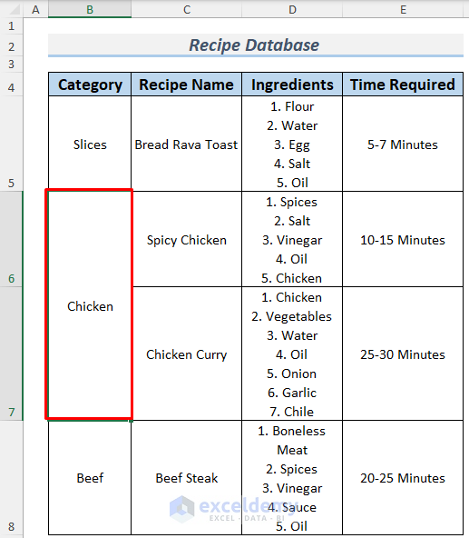
Thus, the cells B6:B7 look merged but they both contain the Category (Chicken).

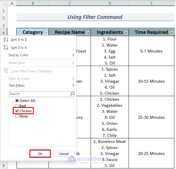
Now, we are ready to use the Filter. Just select the headers (B4:E4) and press CTRL+SHIFT+L. You can find this command from the Editing group of the Home Tab.
Next, the Filter drop-down icons will appear.

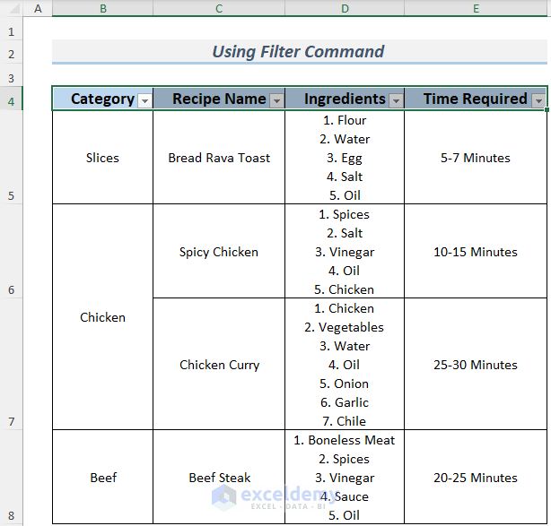
After that, click on the drop-down icon and check the Category you want.
Next, click OK.

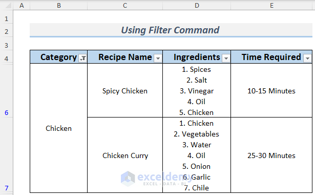
Thus you can Filter your desired items.

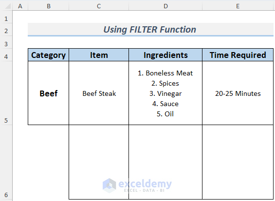
3. Filtering by FILTER Function

We can also use the FILTER function to filter the recipe items. To do that, we have to use Format Painter to format the merged cells as we did in the second filtering method. Also, create the Data Validation following the procedures of the first filtering method. After that, follow the instructions below.

First, select a cell from where your recipe array will start and write down the following formula in it.

=FILTER('recipe list'!C5:E8,'recipe list'!B5:B8=filter!B5,"")

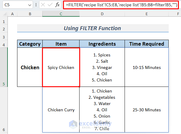
The formula returns the Recipe Item, and corresponding Ingredients and Time Requirements.

Let’s select the Beef category from the Data Validation list and see how this goes.

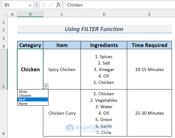
This operation will return the recipe item of the beef category using the formula.

Thus you can create a recipe database in Excel and use it efficiently when it’s needed.

Download Practice Workbook

Recipe Database.xlsx

Conclusion

In the end, we can surmise that you will have an efficient idea of creating a recipe database in Excel after reading this article. If you have any better suggestions, questions, or feedback regarding this article, please share them in the comment box. This will help me enrich my upcoming articles.

<< Go Back To Database in Excel | Learn Excel

Get FREE Advanced Excel Exercises with Solutions!