Watch Video – Create a Relational Database in Excel
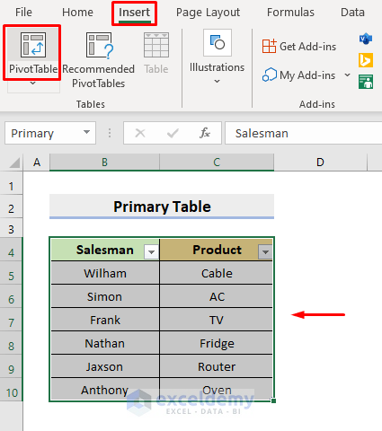
STEP 1 – Build a Primary Table
- Open an Excel worksheet and input your information, as shown in the image below.
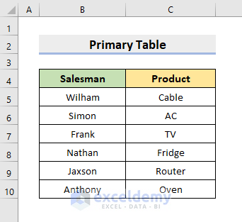
NOTE: You can’t leave an entire row or column blank. Doing so may result in errors in the table.
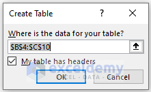
- Select the range B4:C10 and press Ctrl and T together.
- The Create Table dialog box will pop out.
- Press OK
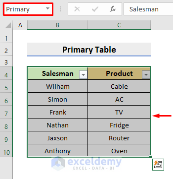
- Select the range and name the table Primary, as shown below.
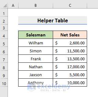
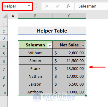
STEP 2 – Form a Helper Table
- Enter the information for the second dataset in a separate worksheet.
- Press keys Ctrl and T simultaneously after selecting the range B4:C10.
- In the pop-up dialog box, press OK.
- Select the range to name the table as Helper.
STEP 3 – Insert Excel Pivot Table
- Select B4:C10 of the Primary table.
- Go to Insert ➤ Pivot Table.
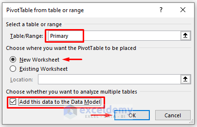
- A dialog box will appear. Select Primary in the Table/Range field.
- Choose a New Worksheet or an Existing Worksheet. Check the box for your selection, as shown below.
- Press OK.
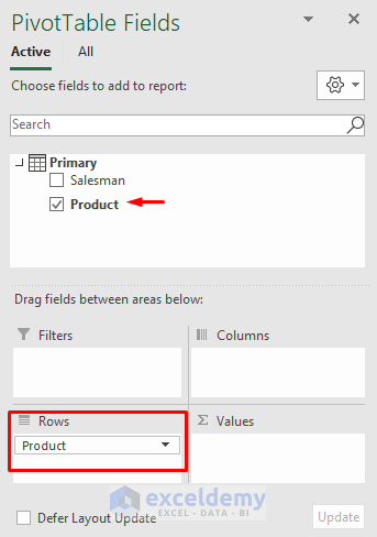
- It’ll return a new worksheet, and on the left side, you’ll see PivotTable Fields.
- Under the Active tab, check the box for Product from Primary and place it in the Rows section, as shown below.
- Go to the All tab.
- Check the box for Net Sales from Table2, which is our Helper table, as shown below.
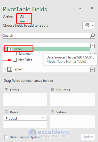
- A yellow-colored dialog will open asking about the relationships between the tables.
- Choose to CREATE.
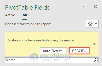
NOTE: You can also click the Auto-Detect option.
- The Create Relationship dialog box will pop out.
- Select Table2 (Helper) in the Table box, and choose Primary in the Related Table field.
- Select Salesman in both the Column fields.
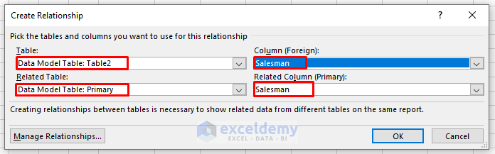
- Press OK.
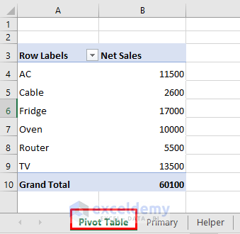
- It’ll return the desired data table in the new worksheet.
Read More: How to Create a Recipe Database in Excel
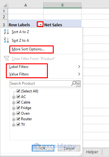
How to Sort and Filter a Relational Database in Excel
STEPS:
- Click the drop-down icon beside the Row Labels header.
- Choose the option that you would like to perform.
How to Update a Relational Database in Excel
STEPS:
- Choose any cell inside the pivot table or the whole range at first.
- Right-click on the mouse.
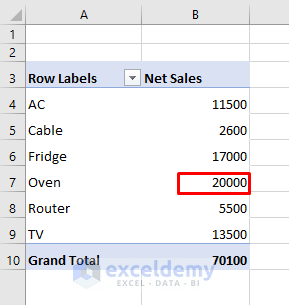
- Select Refresh from the options.
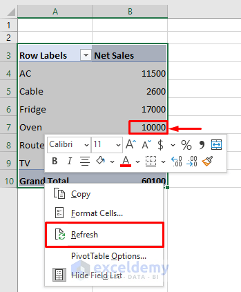
- It’ll return the worksheet updating the data.
Download the following workbook to practice.
Related Articles
- How to Create a Library Database in Excel
- How to Create an Employee Database in Excel
- How to Create a Client Database in Excel
- How to Create Student Database in Excel
<< Go Back To Database in Excel | Learn Excel
Get FREE Advanced Excel Exercises with Solutions!

Great post! I never thought of using Excel for creating a relational database. The three steps you outlined were super helpful and easy to follow. I’m looking forward to trying this out for my project. Thanks for sharing!
Hello Dear,
You are most welcome. Glad to hear that our article helped you to create relational database in Excel. Keep exploring Excel with ExcelDemy!
Regards
ExcelDemy