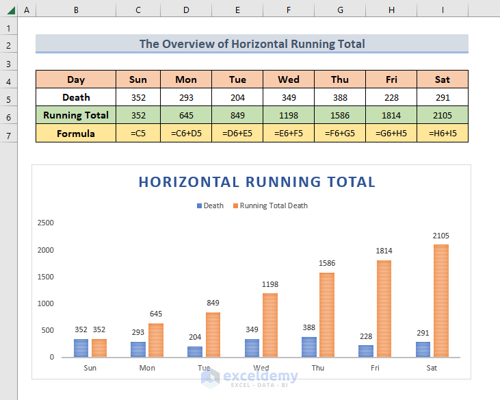
A running total is the total of a series of numbers that updates each time a new number is added to the sequence. It can be calculated by summing up a number with all the previous numbers in the series. In this article, you will learn 3 different methods to calculate the horizontal running total in Excel with each. In the figure below, I have presented an overview image of the Horizontal Running Total.
What is a Running Total
A running total, also known as cumulative total, is the summation of a sequence of numbers which is updated each time a new number is added to the sequence, by adding the value of the new number to the previous running total.
The SUM Function: an Overview
The SUM function is used to add up values altogether. You can use the SUM function, to sum up, distinct values, cell references, ranges, or a mix of all three.
Syntax
SUM(number1,[number2],…)
Arguments
- number1: The first number is required. You can insert general numbers such as 5,7, etc, or cell references like C9, H12, or a cell range like B3:B8.
- number2-255: This field is optional. You can add up to 255 numbers in this field.
Horizontal Running Total in Excel: 3 Ways to Calculate
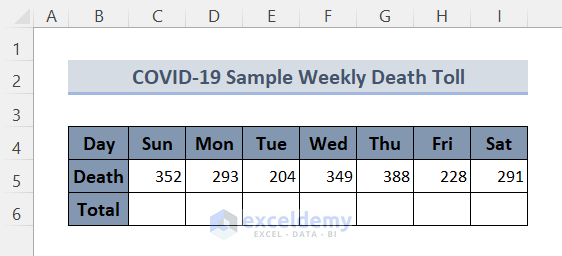
We will be using a Sample COVID-19 Weekly Death Toll as a dataset to demonstrate all 3 methods in this tutorial.
So, without having any further discussion let’s get into all the methods one by one.
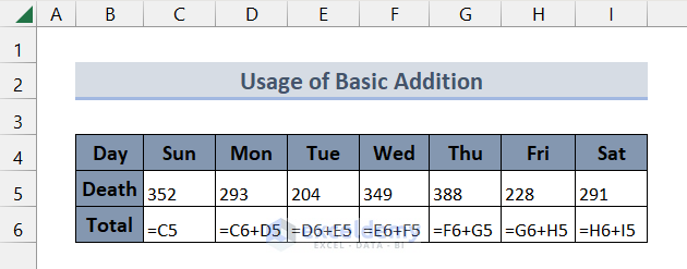
1. Create Horizontal Running Total in Excel Using Basic Addition
We can calculate the horizontal running total in Excel using the basic addition of cell addresses. To learn this method follow the steps below:
🔗 Steps:
The first element of the running total is the death number on the first day of that week. So,
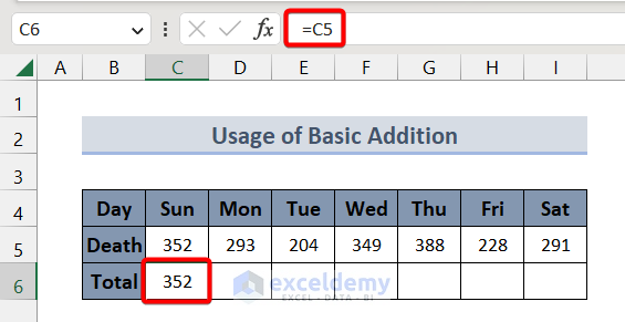
❶ First, select cell C6 and type the following formula within the cell.
=C5❷ Then press the ENTER button. As a result, you will get the value of C5 in C6.
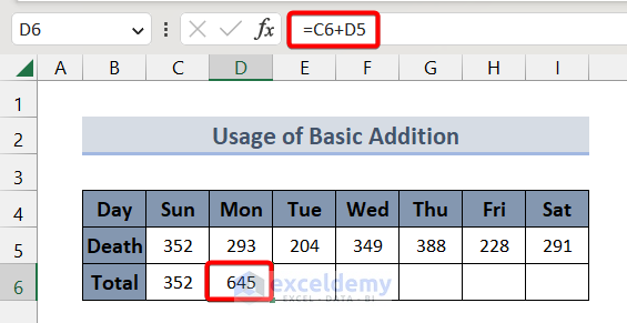
❸ After that select cell D6 and type the following formula.
=C6+D5❹ Then press the ENTER button again. As a result, you will get the sum of death for both Sunday and Monday.
❺ Now all you need to do is drag the Fill Handle icon to the end of the Total row.

That’s it.
📓 Note:
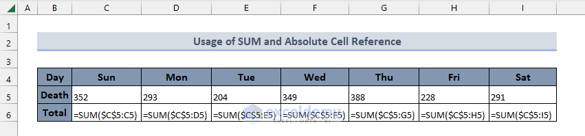
If you feel curious to see all the underlying formulas within the cells then press CTRL + ` keys together. You will see all the formulas as follows afterward:
Read More: How to Calculate Running Total in One Cell in Excel
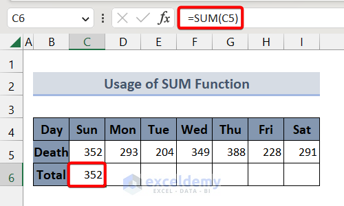
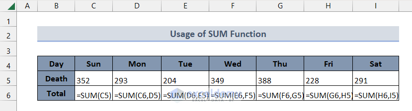
2. Use of SUM Function to Calculate the Horizontal Running Total in Excel
In this section, we will try to avoid the basic addition method. Still, we will apply the same concept but instead of using the plus (+) operator in between cell addresses, we will use the SUM function. Now follow the steps below to get the whole procedure with ease.
🔗 Steps:
❶ First of all, select cell C6.
❷ Then type the following formula.
=SUM(C5)❸ Now, press the ENTER button. As a result, you will get the value of C5.
❹ After that, select cell D6 and type the following formula within the cell.
=SUM(C6,D5)❺ Then press the ENTER button.
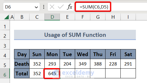
❻ Now drag the Fill Handle icon to the end of the Total row.
That’s it.
📓 Note:
If you feel curious to see all the underlying formulas within the cells then press CTRL + ` keys together. You will see all the formulas as follows afterward:
3. Creating Horizontal Running Total by Using Mixed Cell Reference in Excel
Now, we will discuss the most robust method to create a horizontal running total in Excel using a combination of both the mixed cell reference and relative cell reference. The function we will use in this method is SUM. Now go through the steps below:
🔗 Steps:
❶ First of all, select cell C6 to store the formula result.
❷ After that, type
=SUM($C$5:C5)❸ Then press the ENTER button.
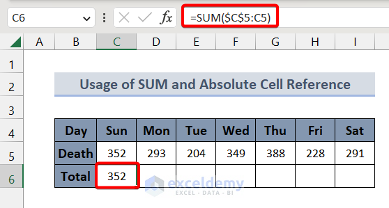
❹ Finally, drag the Fill Handle icon to the end of the Total row.
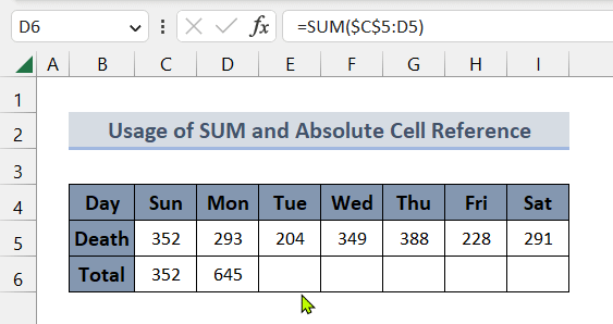
That’s it.
📓 Note:
If you feel curious to see all the underlying formulas within the cells then press CTRL + ` keys together. You will see all the formulas as follows afterward:
Bonus Method: Calculate Vertical Running Total in Excel Using the SUM Function
We can apply the same formula to calculate the vertical running total in Excel. This time we will be using the same formula with the SUM function in this method as in the previous method. Now go through the steps to get it in detail.
🔗 Steps:
❶ First of all, select cell D5 to store the formula result.
❷ After that, type
=SUM($C$5:C5)❸ Then press the ENTER button.

❹ Finally, drag the Fill Handle icon to the end of the Total column.

That’s it.
Read More: Cumulative Sum in Excel If Condition Applied
Things to Remember
📌 You can use CTRL + ` keys to see the cell formulas.
📌 Be careful about the syntax of the function.
📌 Select the cell address range to sum attentively.
Download Practice Workbook
You are recommended to download the Excel file and practice along with it.
Conclusion
To wrap up, we have illustrated 3 different methods overall, to calculate the horizontal running total in Excel. Additionally, we have added an extra method to calculate the vertical cumulative total in Excel. However, you are recommended to download the practice workbook attached along with this article and practice all the methods with that. And don’t hesitate to ask any questions in the comment section below. Surely we will try to respond to all the relevant queries asap.
Related Articles
- How to Create Running Subtraction Total in Excel
- Calculate Running Total by Group Using Excel Power Query
<< Go Back to Excel Running Total | Calculate in Excel | Learn Excel
Get FREE Advanced Excel Exercises with Solutions!
