Method 1 – Using IF with Cell Reference for Excel Cumulative Sum with Condition
Steps:
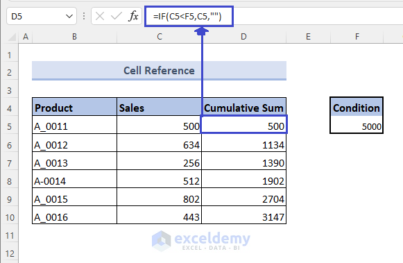
- In cell D5, enter the following formula:
=IF(C5<F5,C5,"")- Press Enter.
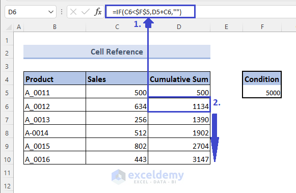
- Enter the following formula in cell D6:
=IF(C6<$F$5,D5+C6,"")- Press Enter.
- Drag the result using the Fill handle until the end of the table.
Formula Breakdown
In the first cell of the result, we used the IF formula, where the logic is the values of sales less than 5000.
Within the IF formula, the return for true is the same as the sales given otherwise blank.
For the second cell of the result, we put the same logic and false return value. The only change is the return for the true value, which will be a summation of the current sales value with the result of the previous cell.
Note: We can find the condition of 5000 in cell F5 and mention this in the formula as an absolute reference.
Read More: How to Calculate Running Total in One Cell in Excel
Method 2 – Using a Header Cell Reference for Excel Cumulative Sum with Condition
Steps:
- Select the modified dataset.
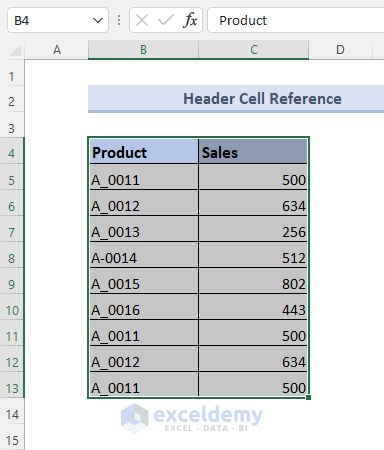
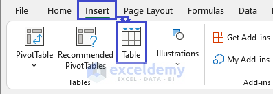
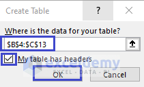
- Select Table from the Insert tab.
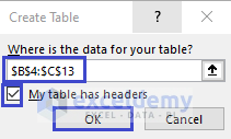
- Check the range of the dataset and tick the My table has headers.
- Click OK.
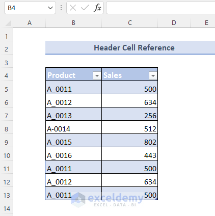
This will create a table with headers and an arrow sign for each, as shown below.
- Choose a new column.
- Enter the following formula in cell D5:
=SUM(Table1[[#Headers],[Sales]]:[@Sales])- Press Enter and drag the result until the end.
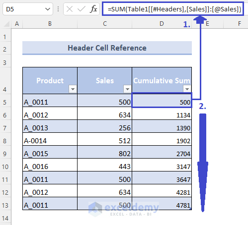
This was the result of the cumulative sum without any condition. It showed results for all the values.
- If we apply the condition, it will show the cumulative sum for repetitive values only.
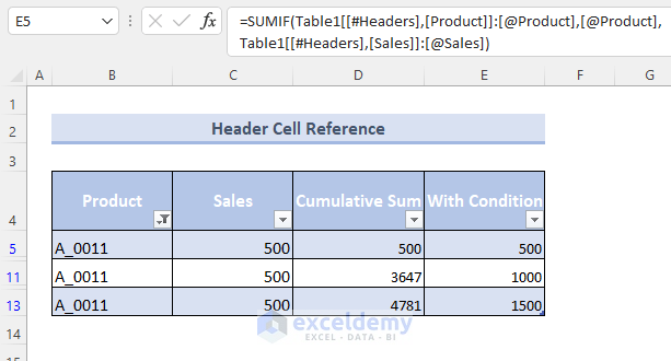
- Enter the following formula in Cell E5:
=SUMIF(Table1[[#Headers],[Product]]:[@Product],[@Product],Table1[[#Headers],[Sales]]:[@Sales])- Press Enter and drag the result using the fill handle to the end of the table.
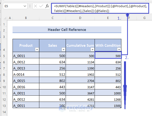
This will show the result of the cumulative sum for repetitive values only.
To see the result of the cumulative sum, you need to follow the steps:
- Right-click the arrow with the Product header, and it will open a drop-down menu.
- Select the product for which you want to see the result.
- Click OK.
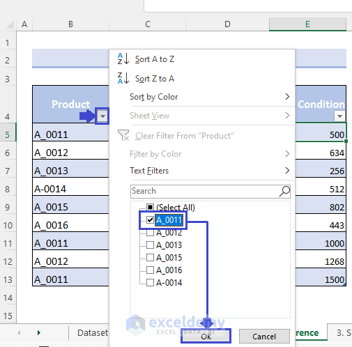
The result will look like this:
Formula Breakdown
Creating the Excel table helped me directly click on headers and cells to refer to the cells without using cell references. It is called table references.
As the SUMIF function takes arguments of sum_range, which is the sales column in our case.
The other arguments include criteria range and criteria from the dataset’s product column.
The first SUMIF formula gave cumulative summation for all the data, while the second one was for the condition that only repetitive values will have the cumulative sum.
Read More: How to Calculate Horizontal Running Total in Excel
Method 3 – Using Nested IF and SUM for Excel Cumulative Sum with Condition
Steps:
- Enter the SUM formula in Cell D5:
=SUM($C$5:C5)- Press Enter to get the result.
- Drag the result to the end of the table.

- If we use the IF formula to keep blank for the results of blank data, enter the formula in Cell E5:
=IF(C5="","",SUM($C$5:C5))- Press Enter and drag the result to where you want.
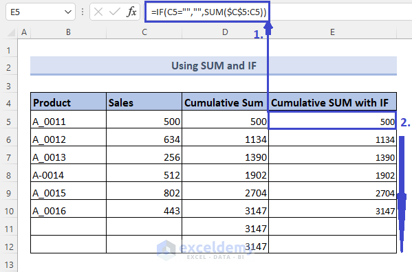
Notice that there are no constant results in blank cells.
Formula Breakdown
The SUM formula uses cell references to give the result of summation.
It gives a constant value for blank cells.
Using the IF formula shows blank results for blank cells and cumulative sum for others.
Method 4 – Using SUM and INDEX for Excel Cumulative Sum If Condition Applied
Steps:
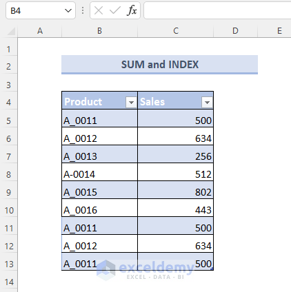
- Select the dataset.
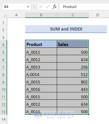
- Choose Table from the Insert tab.

- Check the table range and tick My table has headers option.
- Click OK.
The table will have headers with arrows.
- Enter the following formula in Cell D5:
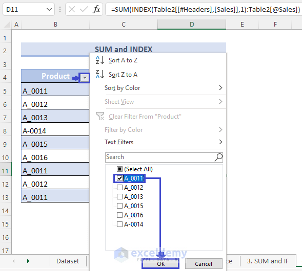
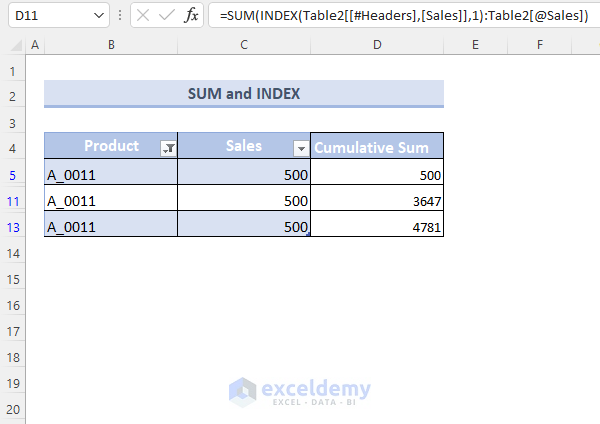
=SUM(INDEX(Table2[[#Headers],[Sales]],1):Table2[@Sales])- Press Enter and drag the result till the end of the table.
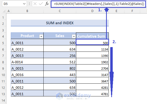
The results will have repetitive values.
This does not consider and give results sequentially.
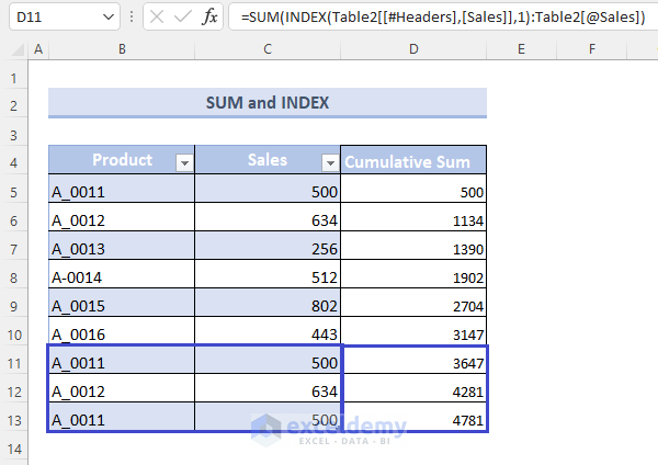
- Right-click on the arrow beside the header of Product and select any of the repetitive products.
- Click OK.
The result is the same.
Formula Breakdown
The INDEX formula uses row and column numbers to find a reference in a range.
After that, it uses the SUM formula to give the summation.
Method 5 – Using SUMIF/SUMIFS for Excel Cumulative Sum with Condition
5.1 Using SUMIF
Steps:
- Enter the following formula in Cell D5:
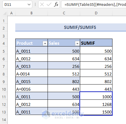
=SUMIF(Table35[[#Headers],[Product]]:Table35[@Product],Table35[@Product],Table35[[#Headers],[Sales]]:Table35[@Sales])- Press Enter and drag the results below.
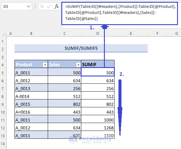
The results are only for the repetitive data.
5.2 Using SUMIFS
Steps:
- Enter the following formula in cell E5:
=SUMIFS(Table35[[#Headers],[Sales]]:Table35[@Sales],Table35[[#Headers],[Product]]:Table35[@Product],Table35[@Product])- Press Enter and drag it using the fill handle.
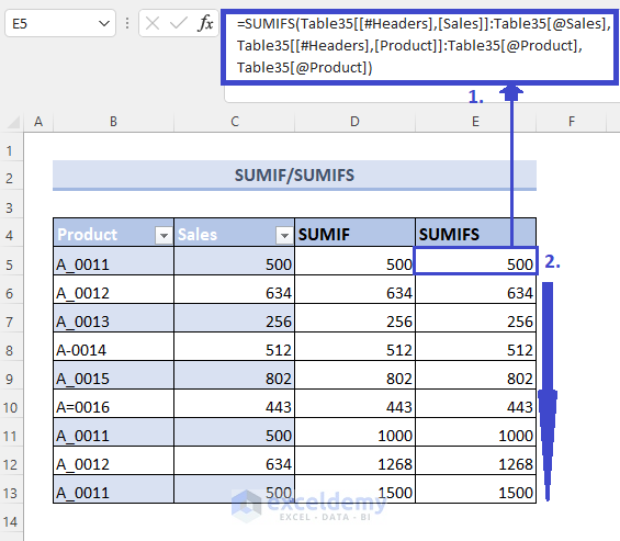
This gives results alike the SUMIF formula.
Method 6 – Using Pivot Table for Excel Cumulative Sum If Condition Applied
Steps:
- Select the modified dataset.
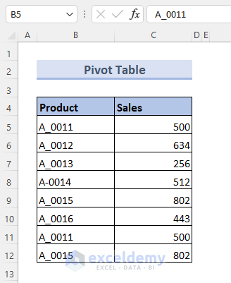
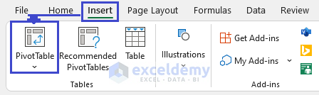
- Select Pivot Table from the Insert tab.
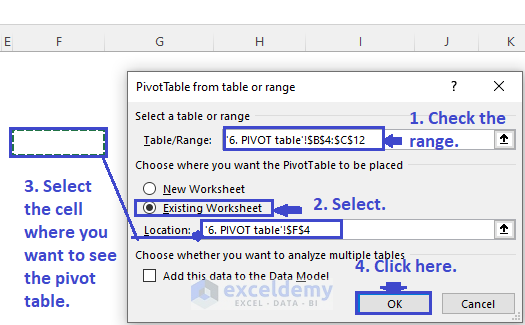
- A new box will open where:
- Check the table range.
- Select Existing Worksheet.
- Select a cell beside the dataset in the Location: section.
- Click OK.
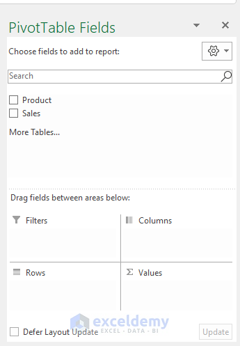
This will open two boxes, one at the selected location and the other on the right side of the sheet. The boxes will look like this.

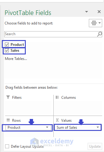
- Tick the Products and Sales. This will be shown in the Rows and Values section, as shown with arrows in the picture below.
- Select the drop-down from the Sum of Sales and click Value Field Settings.
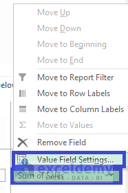
- This will open a new box.
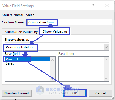
- Enter Cumulative Sum in Custom Name: section.
- Select Show Values As.
- Choose Running Total from the Show values as a drop-down menu.
- Select Product.
- Click OK.
The result will be shown as follows.
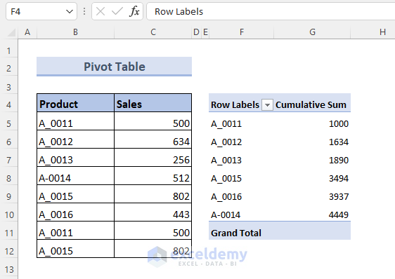
Here, you can see that it adds up the repetitive values and shows only the cumulative sum for the unique product ID.
Download the Practice Workbook
You can download the workbook from the link below.
Related Articles
- Calculate Running Total by Group Using Excel Power Query
- How to Create Running Subtraction Total in Excel
<< Go Back to Excel Running Total | Calculate in Excel | Learn Excel
Get FREE Advanced Excel Exercises with Solutions!
