Microsoft Excel is one of the most beneficial programs you can use. Using Excel’s features and tools, you can do an almost infinite number of things with a dataset. This article will discuss the steps necessary to make a thermometer for a fundraising event. A fundraising thermometer shows us how close we reach a fundraising target. In light of this, the subsequent lesson will focus on the step-by-step process of establishing a fundraising thermometer in Excel.
What Is Fundraising Thermometer?
A fundraising thermometer or thermostat aims to excite donors and raise their contributions to our charity. Most likely, every organization is already familiar with fundraising thermometers. These valuable materials are a standard in the society of nonprofit fundraising professionals. Fundraising thermometers, often known as fundraising target trackers or funding progression bars, display the total amount raised to date.
How to Create a Fundraising Thermometer in Excel ((With Easy Steps))
Establishing a fundraising thermometer in Excel might be challenging if the correct procedures are not followed. This post will lead you through the four steps required to make an Excel thermostat for goal tracking. We will begin by constructing a dataset for this experiment. We will eventually plot the data as a 2D Column Chart. Then, we will build the thermometer using the chart data. Lastly, the Fundraising Thermometer will be tested. Follow these instructions attentively to understand the technique quickly.
Step 1: Set up the Data Model
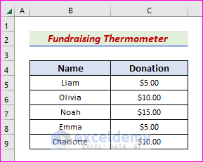
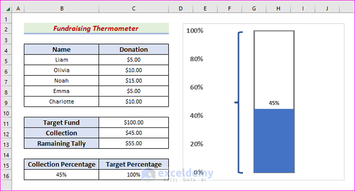
The first and foremost step is to create a dataset for illustration purposes. In this article, we will consider the below dataset. The dataset we will work with has two columns titled Name and Donation. Throughout this step, we will make other necessary information like Target Fund, Collection, and Remaining Tally and columns titled Collection Percentage and Target Percentage for the goal-tracking thermostat.
- First of all, choose the B and C columns.
- Second, make a dataset through the B4:C9 range like the one below.
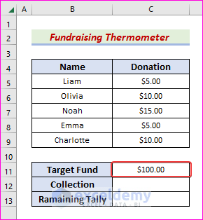
- Third, create three pieces of information through rows 11 to 13 for Target Fund, Collection, and Remaining Tally.
- After that, pick C11 and input 100.
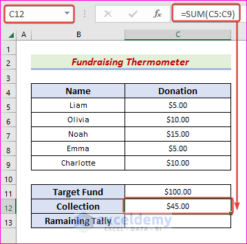
- Presently, select the C12 cell, type the formula below, and hit Enter to see the outcome.
=SUM(C5:C9)
- Likewise, choose the C13 cell and input the formula as follows.
- Later, hit the Enter key to get the output.
=C11-C12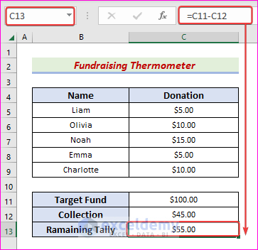
- At this point, build two more columns for the Collection and Target percentages.
- Now, select cell B16, write the formula below, and hit Enter to find the result.
=C12/100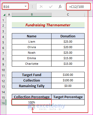
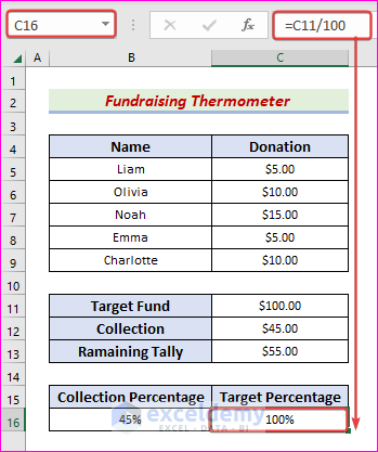
- Later, pick C16, type the formula below and press Enter .
=C11/100
Step 2: Insert Clustered Chart
This step will make a 2D Clustered Chart from the Collection Percentage and Target Percentage columns. Please follow the below instructions to implement the chart.
- First, select the B15:C16 range.
- Secondly, go to the Insert tab and click the Column Chart icon.

- Subsequently, a bar will pop up.
- Now, from the 2-D Column section, choose the 2D Clustered Column symbol.

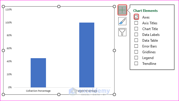
- Consequently, a column chart will appear, and click the Plus icon.
- Later, check only the Axes option.
Step 3: Display Fundraising Thermometer
We will turn the chart data into a simple Thermostat in this context. To accomplish the work, please follow the instructions below.
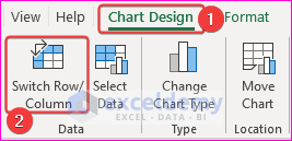
- To begin, click in the chart area and navigate to the Chart Design tab.
- After that, select the Switch Row/Column icon.
- Now, double-click on the Collection Percentage series from the chart.
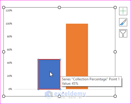
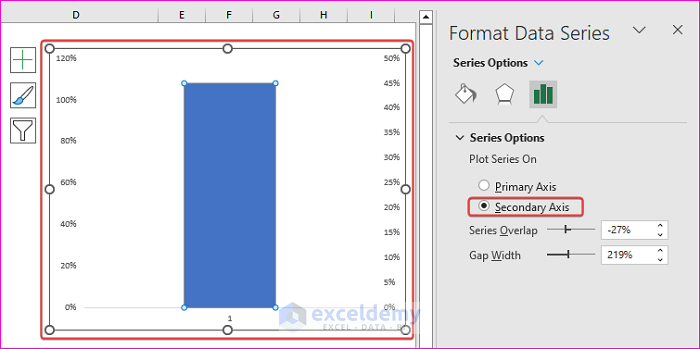
- As a result, the Format Data Series pane will open on the right side.
- Later, check the Secondary Axis from the Series Options to display the chart below.
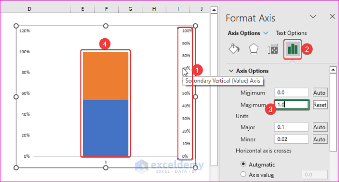
- At this point, double-click on the Secondary Vertical Axis.
- Due to this, the Format Axis pane will pop on the right.
- Now, click the Axis Options and type 1.0 in the box labeled Maximum.
- Then, hit Enter, and the chart will look like the below one.
- Presently, select the Secondary Axis again and press Backspace.
- As a consequence, the Secondary Axis will disappear.
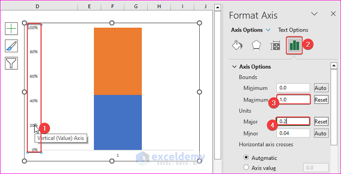
- Latterly, double-click the Vertical Axis, and the Format Axis pane will open.
- Then, click on the Axis Options icon and type 0 in the Maximum box.
- Next, write 2 in the box labeled Major and hit Enter.
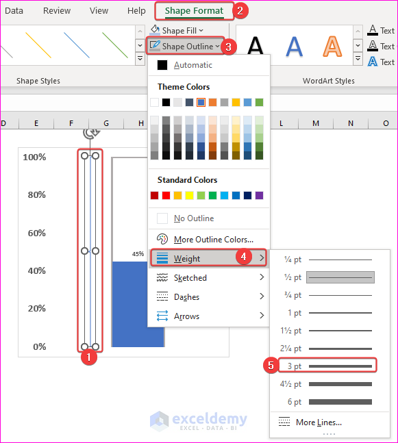
- At this point, click the Target Percentage Value.
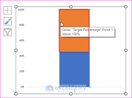
- Then, go to the Format tab and click the Shape Styles symbol.
- Later, from the Shape Fill option, choose the White color.

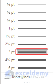
- Later, click the Shape Outline option and choose Weight.
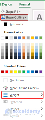
- Afterward, select the 3pt option.
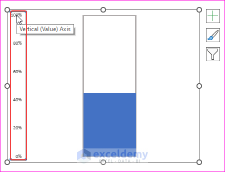
- Eventually, pick the Horizontal Axis and tap Backspace.

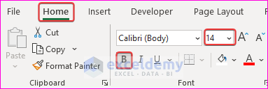
- Presently, click on the Vertical Axis.
- Later, navigate to the Home Choose the B icon from the Font group and make the Font size 14.
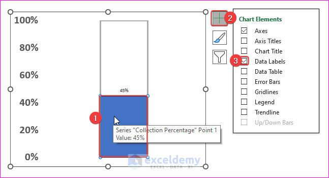
- Now, pick the Collection Percentage series, click on the Plus symbol, and check the Data Labels.
- After that, go to the Insert tab and choose the Shapes symbol.

- Then, from the Basic Shapes, select the Left Brace.

- Currently, draw the Left Brace right beside the thermometer.
- Latterly, go to the Shape Format tab, and click on,
Shape Format → Shape Outline → Weight → 3pt
- As a result, the thermometer will look like the below one.
Step 4: Test Fundraising Thermometer
Now, we will test the fundraising thermometer. We will increase their donation and track the thermostat for every name listed in the dataset.
- First of all, select the C5:C9 range and press Delete.
- Second, pick the C5 cell, type 20, and hit Enter.
- Likewise, input 20 to all other cells and notice the changes in the thermometer.
- Thus, we created a fundraising thermometer like the below one.
Download Practice Workbook
Please click on the link below this paragraph if you want a free copy of the sample workbook discussed in the presentation.
Conclusion
You can make a fundraising thermometer in Excel by following our steps. Please feel free to add comments, suggestions, or questions in the section below if you have any confusion or face any problems. We will try our best to solve the problem or work with your suggestions.
Related Articles
- How to Create a Thermometer Chart in Excel
- How to Create Goal Thermometer Excel
- How to Create Debt Thermometer Excel
- How to Create Progress Thermometer in Excel
<< Go Back To Thermometer Chart in Excel | Excel Charts | Learn Excel
Get FREE Advanced Excel Exercises with Solutions!
