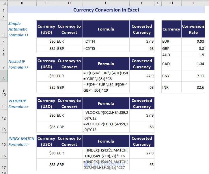
We have some currencies in USD. We’ll convert them to Euro and GBP.
⏷Simple Arithmetic Formula for Currency Conversion
⏷Currency Conversion by Applying Nested IF Function
⏷Using the VLOOKUP Function
⏷Using INDEX MATCH to Convert Currency
⏷Currencies Data Type to Create Currency Converter
⏷Converting Currency Using Web Query
⏷Automate Currency Conversion Using VBA
⏷How to Change Default Currency in Excel?
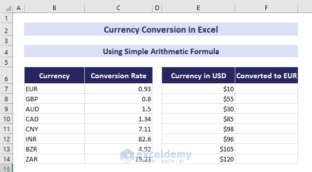
Method 1 – Using a Simple Arithmetic Formula for Currency Conversion in Excel
We have some amounts in USD in column E, a list of currencies in the range B7:B14 and their corresponding conversion rate with respect to USD in C7:C14. Let’s convert USD to EUR in Excel.
Steps:
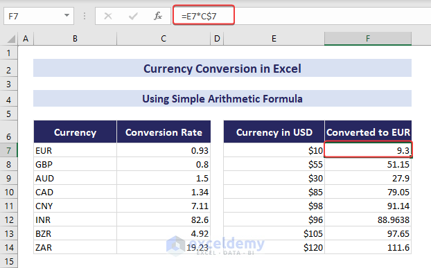
- Select cell F7 and insert the formula:
=E7*C$7- Press Enter. It will return the EUR currency equivalent to the USD currency value.
- Use the Fill Handle tool to copy the formula to the cells below.
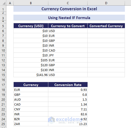
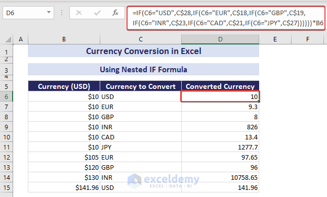
Method 2 – Currency Conversion in Excel by Applying a Nested IF Function
We have currency amounts in USD in the range B6:B15. We have kept different currencies and their corresponding conversion rates from USD to other currencies in the range B18:C25.
Steps:
- Select cell D6.
- Insert the following formula:
=IF(C6="USD",C$28,IF(C6="EUR",C$18,IF(C6="GBP",C$19, IF(C6="INR",C$23,IF(C6="CAD",C$21,IF(C6="JPY",C$27))))))*B6- Press Enter and use the Fill Handle tool to fill the column.
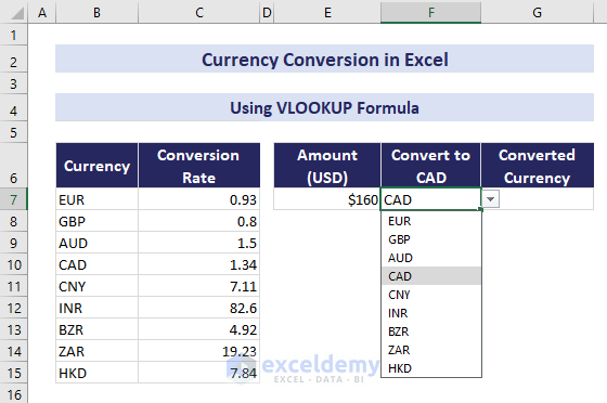
Method 3 – Using the VLOOKUP Function to Convert Currency in Excel
We have a list of currencies in column B and conversion rates in column C. In cell F7, we made a drop-down list with the currency names. We will select a currency from the drop-down list and get the output in cell G7 with the converted currency amounts.
- Insert the following formula in G7:
=VLOOKUP(F7,B7:C15,2,0)*E7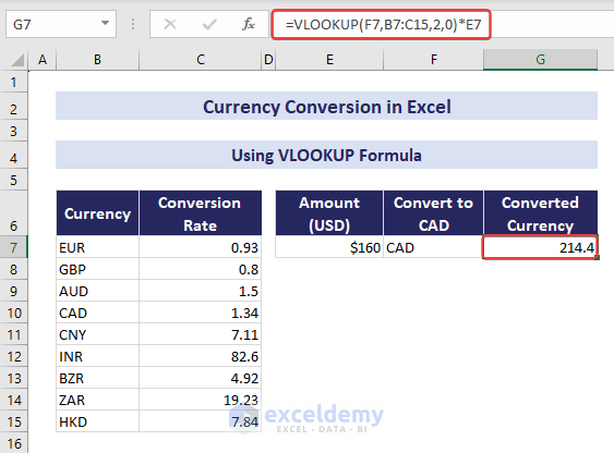
- Changing the currency from the drop-down changes the result.
Method 4 – Using INDEX-MATCH to Convert Currency in Excel
- Use the following formula in G7:
=(INDEX(B7:C15,MATCH(F7,B7:B15,0),2))*E7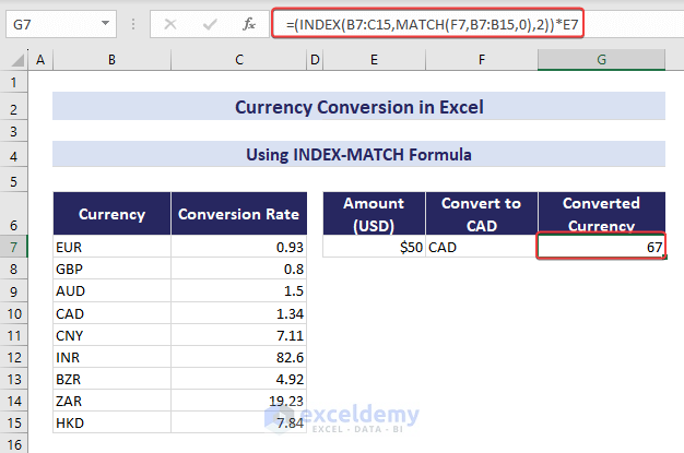
- If you change the values in E7 (amount) and F7 (currency), the result will change.
Read More: How to Convert Text to Currency in Excel
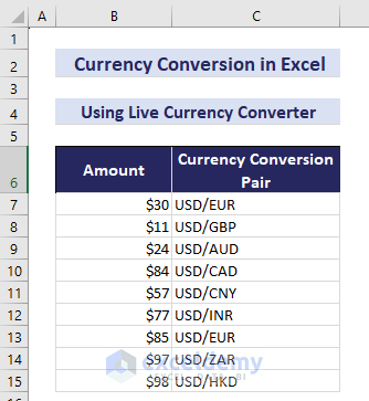
Method 5 – Using the Currencies Data Type to Create a Currency Converter in Excel
Converting currencies using the Currencies data type feature is only available in Microsoft 365.
In our dataset, column B contains currency in USD, and column C contains the currency conversion pair. They are in the form of currency before and currency after. For example, the USD/EUR pair means we will convert USD to EUR currency.
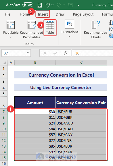
Steps:
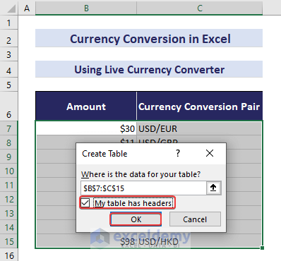
- Select the whole range (B7:C15).
- Go to the Insert tab and click on Table (Alternatively, press Ctrl + T).
- The Create Table dialog box will appear.
- Check the box My table has headers.
- Click OK.
- Select the range C7:C15.
- Go to the Data tab.
- Click Currencies from the Data Types section.
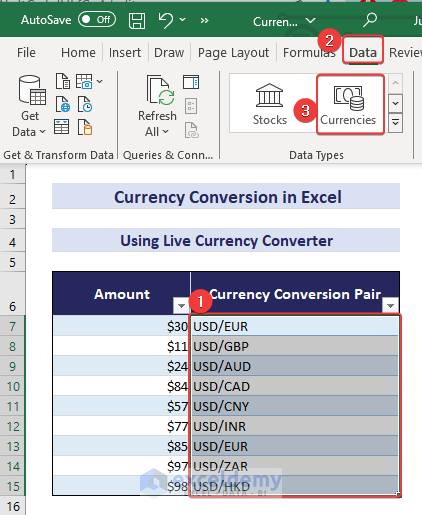
- A new symbol has appeared before all the pairs in Column C.
- Select the range C7:C15.
- Click on the Add Column option.
- Select Price to get the conversion rates in a new column.
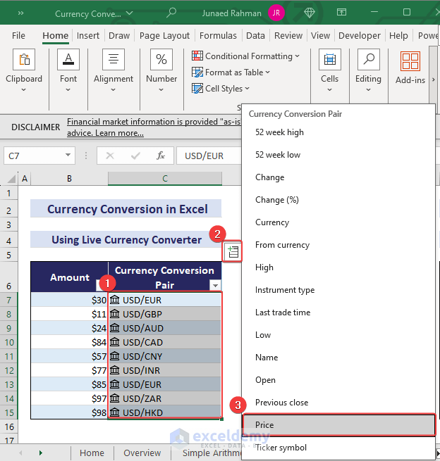
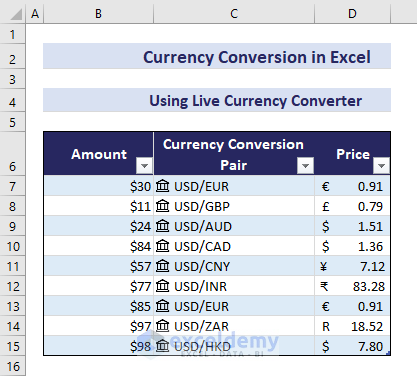
- We will get the conversion rates in Column D.
You can add a new column that contains the last time a currency was updated.
- Select C7.
- Click on the Add Column option.
- Select Last trade time.
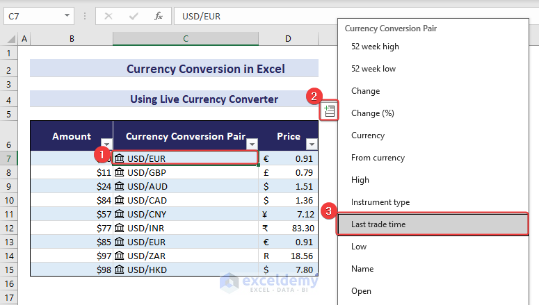
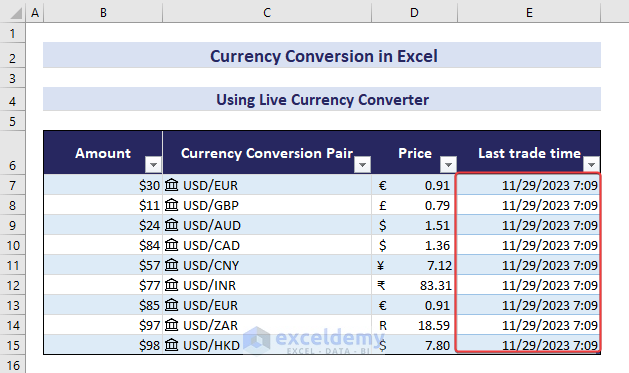
- You will get the following output in column E, containing the last trade time of the currencies (11/29/2023, 7:09)
- Apply the following formula in cell F7 to find the converted currency amounts.
=[@Amount]*[@Price]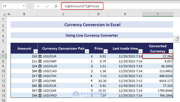
Read More: How to Automate Currency Conversion in Excel
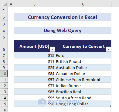
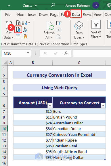
Method 6 – Converting Currency in Excel Using Web Query
In our dataset, Column B contains some amounts in USD, and Column C contains the desired currencies we want to convert into.
Steps:
- Click the Data tab.
- Select From Web in the Get & Transform Data group.
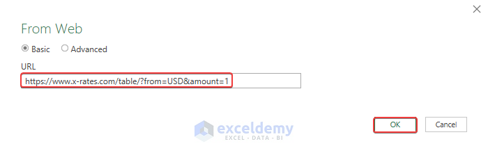
- In the From Web dialog box, paste the following website link and click OK.
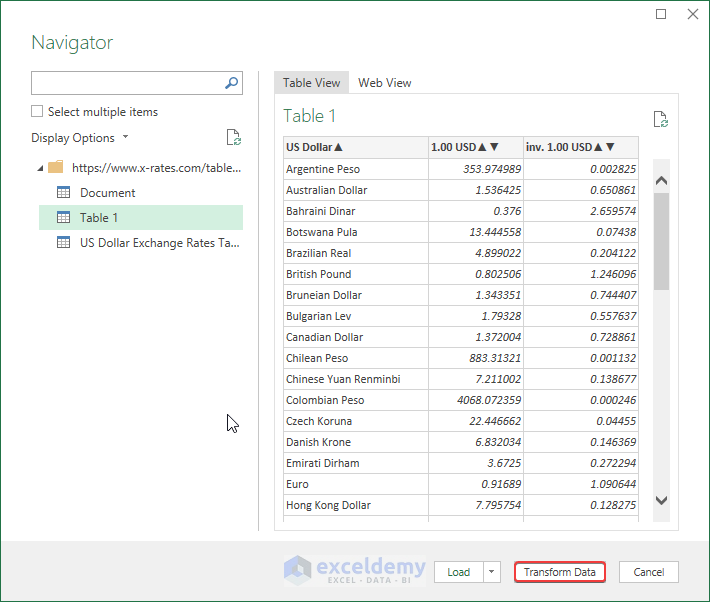
- The Navigator window will open. Choose the table that needs to be loaded.
- After selecting Table 1 in the left pane, click on Transform Data.
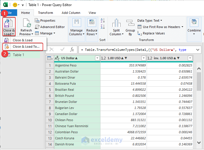
- The table will be loaded in the Power Query Editor.
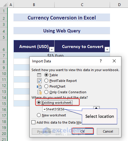
- In the Power Query Editor, click Close & Load and choose Close & Load To…
- The Import Data dialog box will appear.
- Select the option Existing worksheet.
- Select a location in the sheet.
- Press OK.
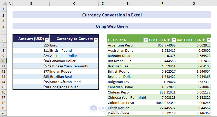
The table will appear in the desired location, as shown in the image below. The first column of the table contains the name of the currency. The second column contains the conversion rate from USD to the corresponding currency. The last column contains the reverse conversion rate, the rate from any currency to USD. The exchange rates were taken on 11/29/2023 while writing this article.
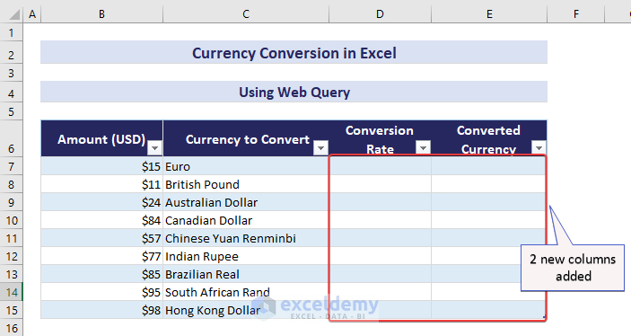
- Add two new columns after column C. Name column D as Conversion Rate and column E as Converted Currency.
- In cell D7, use the following formula to calculate the conversion rate:
=VLOOKUP([@[ Currency to Convert]],Table_1,2,0)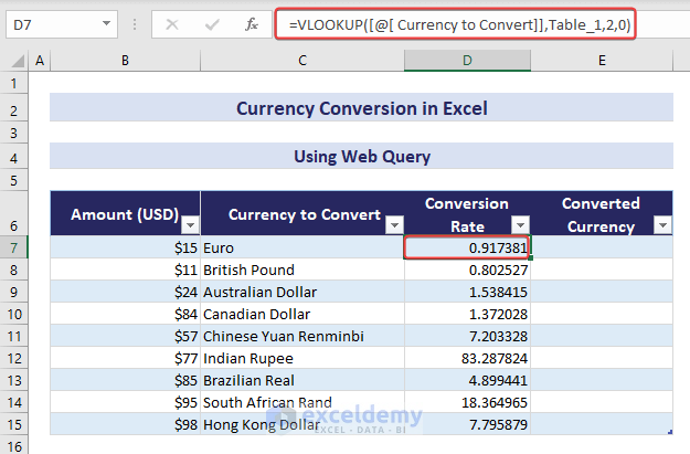
- Apply the following formula in column E to get the converted currencies:
=[@[Amount (USD)]]*[@[Conversion Rate]]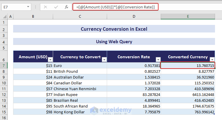
Method 7 – Automate Currency Conversion in Excel Using VBA
Steps:
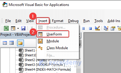
- Press Alt + F11 to open the VBA editor.
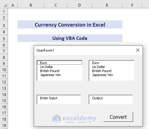
- Click Insert and select UserForm to get a blank user form to edit.
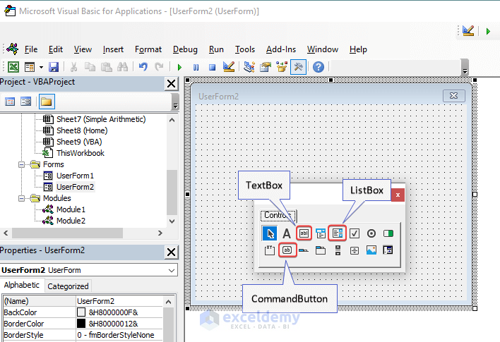
- Use the Toolbox of the UserForm to insert various elements.
- Insert two ListBoxes in the upper portion of the UserForm and two TextBoxes in the lower portion of the UserForm.
- Insert a CommandButton in the lower right portion of the UserForm.
- Give an appropriate name to the CommandButton.
- Right-click on the button.
- Select View Code.
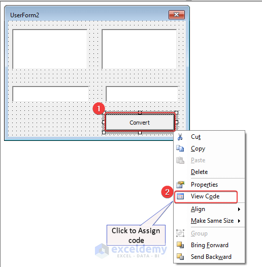
- Copy and paste the following code into the UserForm code window:
Private Sub CommandButton1_Click()
' Conversion ex_rates matrix
Dim ex_rates() As Variant
ex_rates = Array(Array(1, 1.38475, 0.87452, 163.83), _
Array(0.722152, 1, 0.63161, 150.62), _
Array(1.143484, 1.583255, 1, 188.16), _
Array(1.143484, 0.0066, 0.0053, 1))
' Get selected indices from ListBoxes
Dim x As Integer, y As Integer
x = ListBox1.ListIndex
y = ListBox2.ListIndex
' Check if both indices are selected
If x >= 0 And y >= 0 Then
' Perform conversion and update TextBox2
TextBox2.Value = TextBox1.Value * ex_rates(x)(y)
End If
End Sub- Assign the associated code to the UserForm_Initialize section of the same window.
Private Sub UserForm_Initialize()
With ListBox1
.AddItem "Euro"
.AddItem "Us Dollar"
.AddItem "British Pound"
.AddItem "Japanese Yen"
End With
With ListBox2
.AddItem "Euro"
.AddItem "Us Dollar"
.AddItem "British Pound"
.AddItem "Japanese Yen"
End With
TextBox1.Value = "Enter Input"
TextBox2.Value = "Output"
End Sub- Assign the following codes in the same code window to make the ListBoxes and TextBox1 dynamic.
Private Sub TextBox1_Change()
TextBox2.Text = ""
End Sub

Private Sub ListBox2_Change()
TextBox2.Text = ""
End Sub

Private Sub ListBox1_Change()
TextBox2.Text = ""
End Sub- Add the following code in the same window.
Private Sub TextBox1_Enter()
'This code runs when the user clicks on TextBox1
'Check if the current text is "Enter Amount"
  If TextBox1.Value = "Enter Input" Then
    'Clear the text and make it a null textbox
    TextBox1.Value = ""
    TextBox2.Value = ""
  End If
End Sub
Our UserForm is ready to use now.
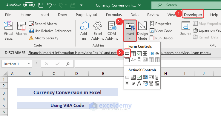
We will insert a button in the worksheet.
- Go to Developer and select Insert, then choose Button (under Form Controls).
- To assign a Macro to the button, right-click on the button, select Assign Macro, and paste the following code.
Sub Button1_Click()
UserForm1.Show
End Sub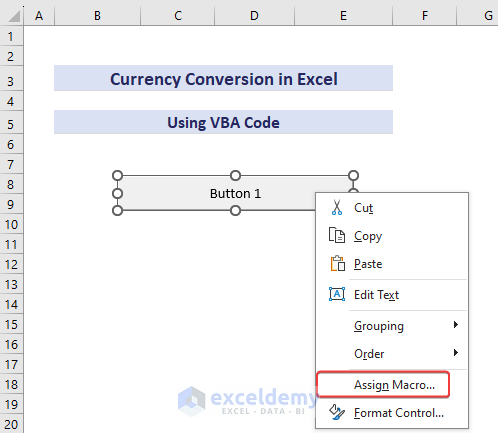
- Click on the button and you’ll get a UserForm as a calculator.
How to Change the Default Currency in Excel?
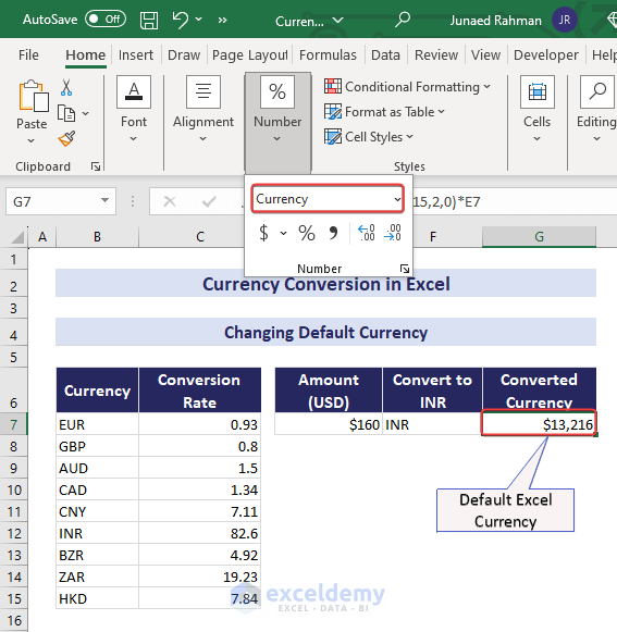
The following image shows a currency amount in cell G7. Excel has automatically considered it to be USD. But, we want it to change it to INR.
Steps:
- Select the cell G7.
- Click Number group in Home tab.
- Click the Number Format symbol.
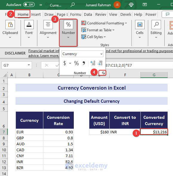
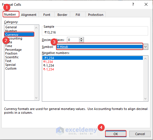
- This will open the Format Cells dialog box.
- Select Number then Currency.
- Select the desired currency from the Symbol: drop-down menu.
- Click OK.
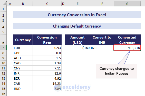
- The currency symbol has been changed to INR.
Read More: How to Change Default Currency in Excel
Download the Practice Workbook
Currency Conversion in Excel: Knowledge Hub
<< Go Back to Learn Excel
Get FREE Advanced Excel Exercises with Solutions!
