Method 1 – Automate Currency Conversion Using Multiplication
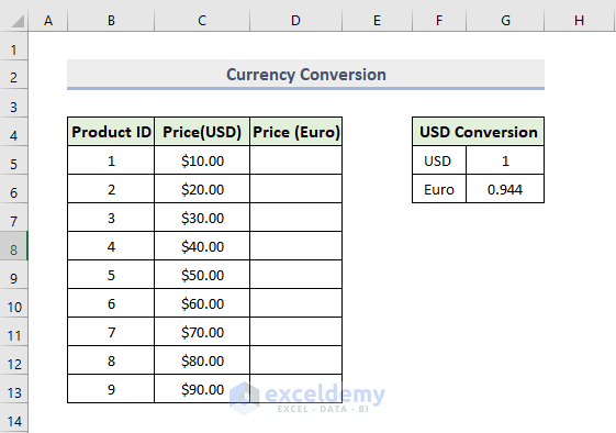
We have a sample dataset where the price of each product is shown in USD, which we want to convert to EURO.
Steps:
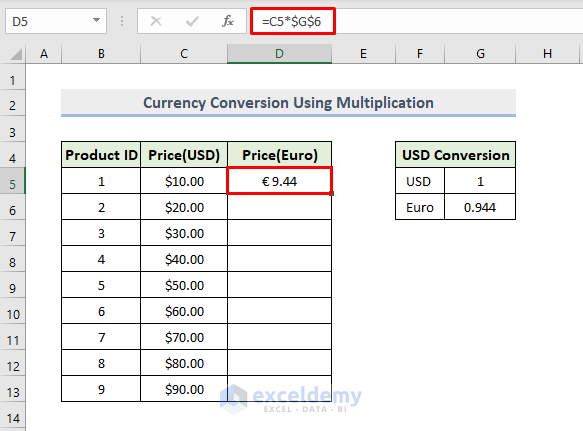
- Use the following formula in cell D5:
=C5*$G$6
Here, cell G6 is the conversion rate of USD to EURO.
- Press Enter.
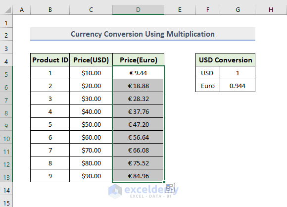
- Drag the Fill handle icon.
- The price will convert from USD to EURO.
Method 2 – Utilizing Nested IF Formula to Automate Currency Conversion
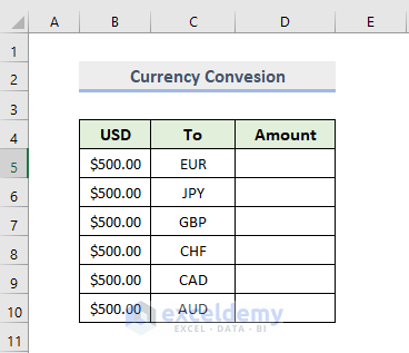
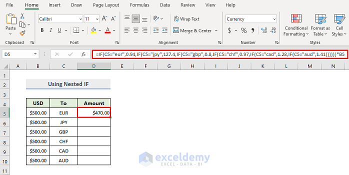
In the following dataset, we want to convert USD to different currencies such as EUR, JPY, GBP, CHF, CAD, and AUD.
Steps:
- Use the following formula in cell D5:
=IF(C5="eur",0.94,IF(C5="jpy",127.4,IF(C5="gbp",0.8,IF(C5="chf",0.97,IF(C5="cad",1.28,IF(C5="aud",1.41))))))*B5
- Press Enter.
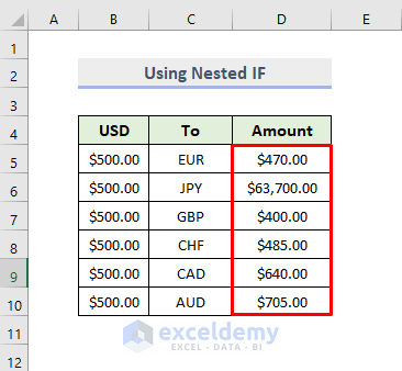
- Drag the Fill handle icon.
- The amount will be converted from USD to the different currencies entered.
How Does the Formula Work?
- Here, we define a condition whether cell C5 is equal to EUR, JPY, GBP, CHF, CAD, or AUD. Once this condition is met, the function will return a value and the value will be multiplied by cell B5.
Method 3 – Using VLOOKUP Function to Automate Currency Conversion
Steps:
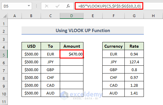
- Use the following formula in the cell D5:
=B5*VLOOKUP(C5,$F$5:$G$10,2,0)
- Press Enter.
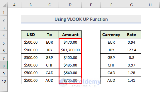
- Drag the Fill handle icon.
- The amount will be converted from USD to the different currencies entered.
How Does the Formula Work?
- The VLOOKUP function looks for a value in the table array F5:G10 and then returns a value in the row from the column we specify.
- The returned value is multiplied by cell B5 to give the converted amounts for each currency.
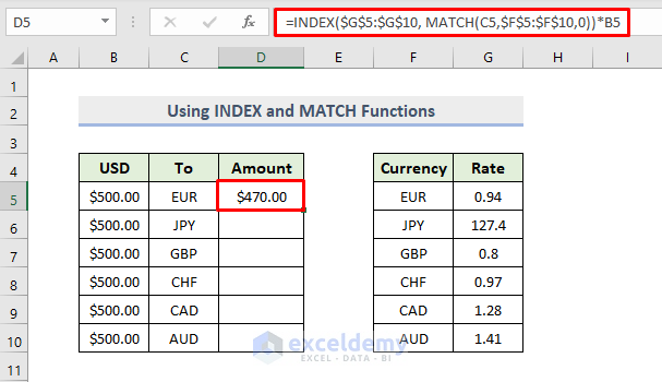
Method 4 – Combination of INDEX and MATCH Functions in Excel
Steps:
- Use the following formula in cell D5:
=INDEX($G$5:$G$10, MATCH(C5,$F$5:$F$10,0))*B5
- Press Enter.
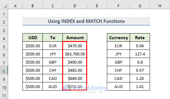
- Drag the Fill handle icon.
- The amount will be converted from USD to the different currencies entered.
How Does the Formula Work?
- The MATCH(C5,$F$5:$F$10,0) function returns the relative position of an item in the array F5:F10 that matches a specified value C5 in the specified order.
- The INDEX function returns the 0.94 which is in the first row of the range F5:F10.
- Multiply the whole combined functions by cell B5 to get the final output.
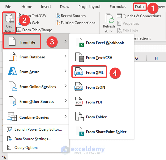
Method 5 – Using External XML Source in Excel
Steps:
- Go to the Data tab, select Get Data > From File > From XML.
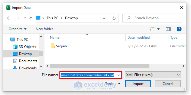
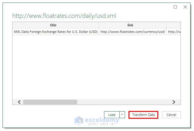
- When the Import Data window appears, enter the URL: http://www.floatrates.com/daily/usd.xml in the File name. Then, click on Import.
- Click on Transform Data.
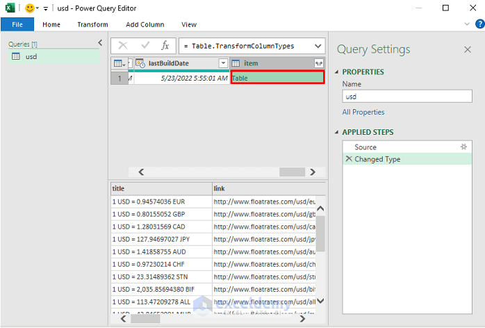
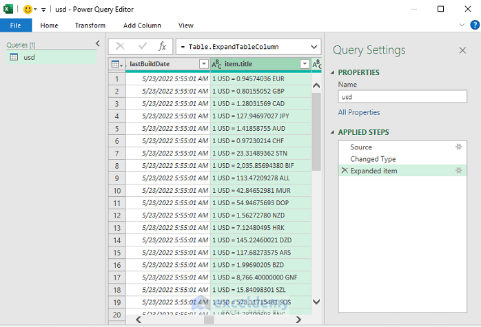
- When the Power Query Editor opens, go to the Item. Click on Table.
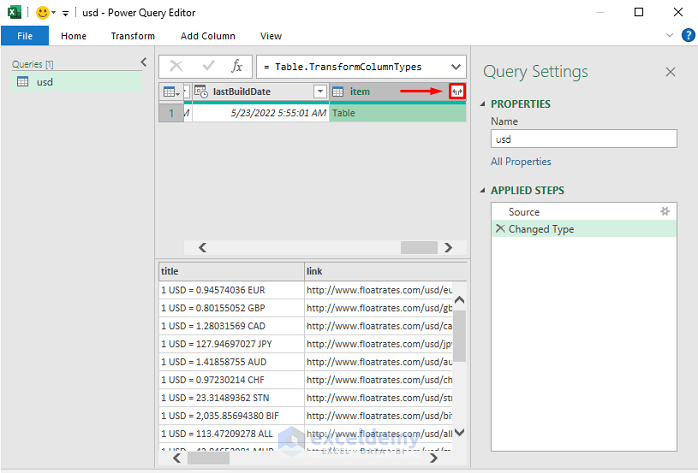
- Click on the arrow.
- Click on OK.
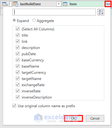
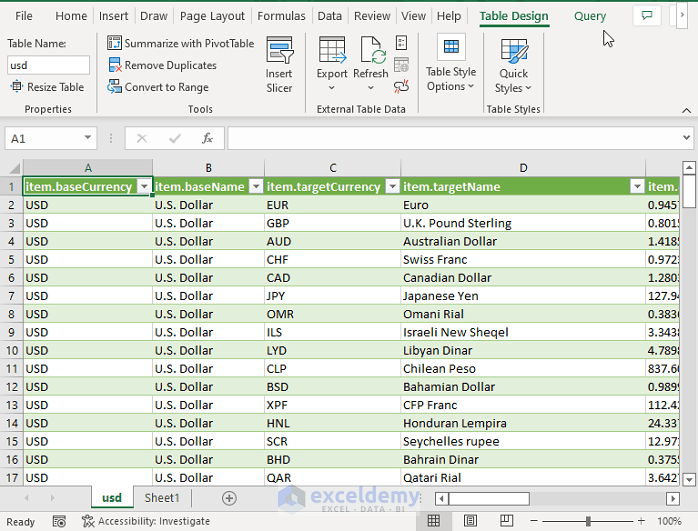
- You will get the exchange rate columns.
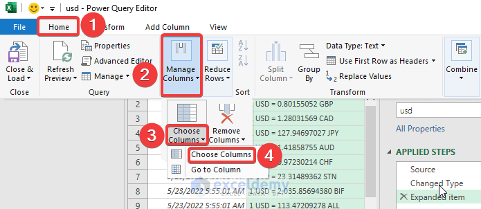
- Select Home > Manage Columns > Choose Columns.
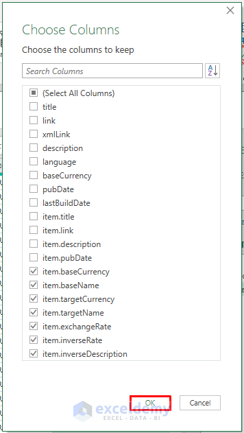
- Check the required columns like the following and click on OK.
- Click on Close & Load.
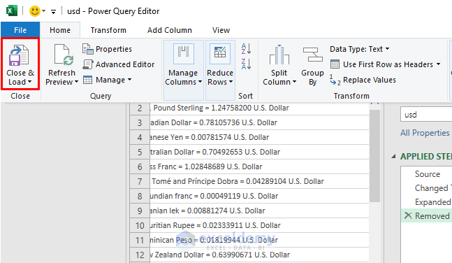
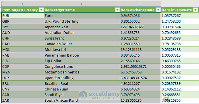
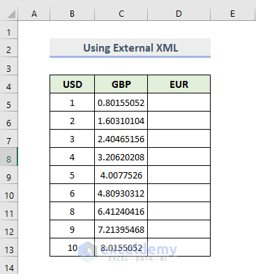
- You will get the exchange rate in the spreadsheet.
- Now, you have to create a new worksheet
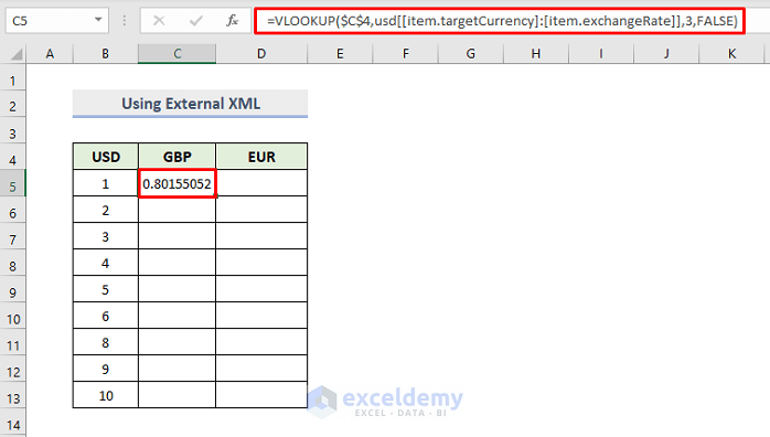
- Use the following formula in the cell C5:
=VLOOKUP($C$4,usd[[item.targetCurrency]:[item.exchangeRate]],3,FALSE)
Here, C4 is the GBP currency and the final argument is False.
- Press Enter.
- The [[item.targetCurrency]:[item.exchangeRate]] is the lookup data in the linked XML file.
- Use the following formula in cell C6:
<span style="color: #000000;">=VLOOKUP($C$4,usd[[item.targetCurrency]:[item.exchangeRate]],3,FALSE)*B6</span>
Here, C4 is the GBP currency and the final argument is False. The whole formula is multiplied by cell B6 to get the converted currency.
- Press Enter.
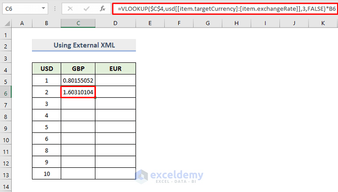
- Drag the Fill handle icon.
- It will convert USD TO GBP.
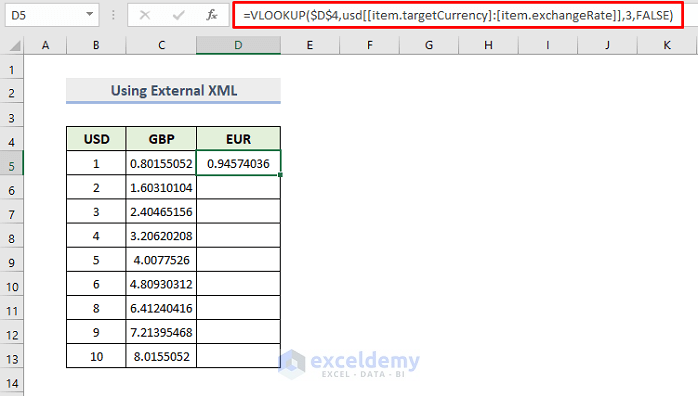
- Use the following formula in the cell D5:
<span style="color: #000000;">=VLOOKUP($D$4,usd[[item.targetCurrency]:[item.exchangeRate]],3,FALSE)</span>
Here, D4 is the EUR currency and the final argument is False. The [[item.targetCurrency]:[item.exchangeRate]] is the lookup data in the linked XML file.
- Press Enter.
- Use the following formula in the cell D6:
=VLOOKUP($D$4,usd[[item.targetCurrency]:[item.exchangeRate]],3,FALSE)*B6
Here, C4 is the GBP currency and the final argument is False. The whole formula is multiplied by cell B6 to get the converted currency.
- Press Enter.
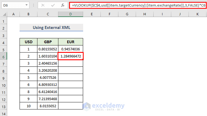
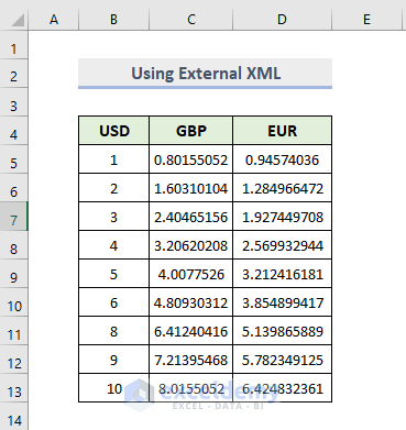
- Drag the Fill handle icon.
- It will convert USD to different currencies.
Download Practice Workbook
<< Go Back to Currency Conversion in Excel | Learn Excel
Get FREE Advanced Excel Exercises with Solutions!
