How to Make a Forecasting Balance Sheet in Excel (With 3 Steps)

Creating a balance sheet is a prerequisite for performing financial analysis and evaluating an individual or organization. However, we may want to forecast financial performance based on historical data because it can provide a valuable understanding of an organization’s financial strengths and weaknesses. Keeping this in mind, this article explains how to make a forecasting balance sheet in Excel.

Download Practice Workbook

3 Steps to Make a Forecasting Balance Sheet in Excel

First of all, let’s consider the Assumptions illustrated in the B4:F15 cells. Following this, we’ll prepare a forecasting balance sheet for the years 2022, 2023, 2024, and 2025 while considering that we have the following data as shown in the Assumptions.

Now, the screenshot below shows a bird’s eye view of the completed forecasting balance sheet. Therefore, without further delay, let’s see the process in detail.

Here, we have used the Microsoft Excel 365 version, you may use any other version according to your convenience.

📌 Step 1: Enter the Assets

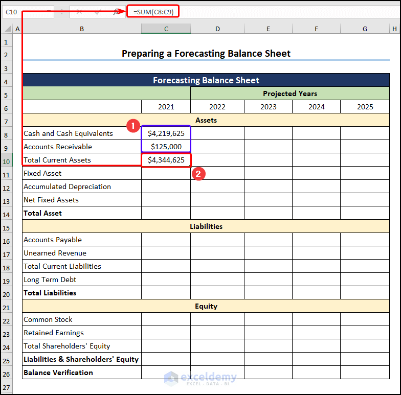
• First, enter the Cash and Cash Equivalents and the Accounts Receivable in the C8 and C9 cells respectively.
• Next, go to the C10 cell and use the SUM function as shown below.

Here, C8 and C9 cells refer to the values of $4,219,625 and $125,000.

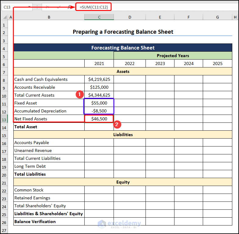
• Now, enter the Fixed Asset and Accumulated Depreciation in the C11 and C12 cells respectively >> calculate the Net Fixed Assets using the formula given below.

In this case, the C11 and C12 cells represent the values of $55,000 and -$8,500 respectively.

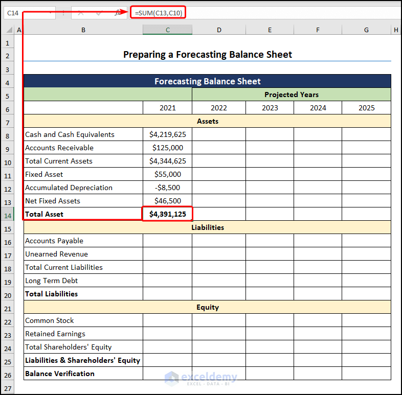
• Then, obtain the Total Asset by adding the Total Current Assets and the Next Fixed Assets.

In the above equation, C10 and C13 cells point to the values of $4,344,625 and $46,500.

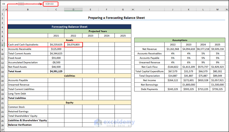
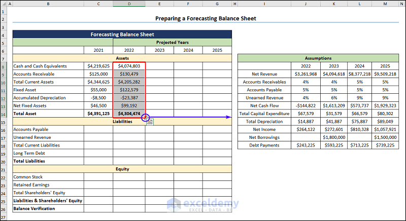
• Second, move to the D8 cell >> and insert the following expression.

Here, the C8 and J18 cells represent the Cash and Cash Equivalents for 2021 ($4,219,625) and the Net Cash Flow (-$144,822) values, respectively.

• In the next step, compute the Account Receivable using the expression given below.

Here, J9 and J10 cells refer to the Net Revenue ($3,261,968) and the assumed Account Receivable (4%) for the year 2022.

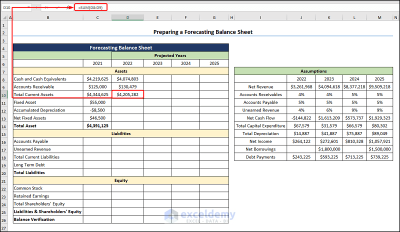
• Now, calculate the Total Current Assets as shown previously.

In this equation, D8 and D9 cells refer to the values of $4,074,803 and $130,479.

• Following this, obtain the Fixed Asset using the expression given below.

In this expression, the C11 cell represents the Fixed Asset ($55,00) for 2021 while the J14 cell refers to the assumed Total Capital Expenditure of $67,579.

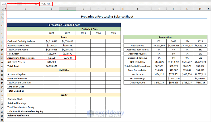
• In turn, calculate the Accumulated Depreciation by utilizing the formula given below.

Here, the C12 cell indicates the Accumulated Depreciation for the year 2021 (-$8,500) and the J15 cell represents the assumed Total Depreciation ($14,887) respectively.

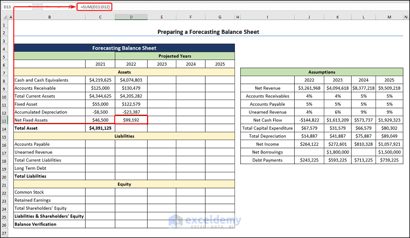
• Following this, get the Net Fixed Assets for the year 2022 by applying the following expression.

In the above equation, D11 and D12 cells point to the Fixed Asset ($122,579) and Accumulated Depreciation (-$23,387).

• Finally, obtain the Total Asset by inserting the following equation.

In this equation, the D13 and D10 cells indicate the Net Fixed Assets ($99,192)and Total Current Assets ($4,205,282).

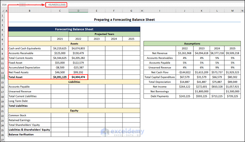
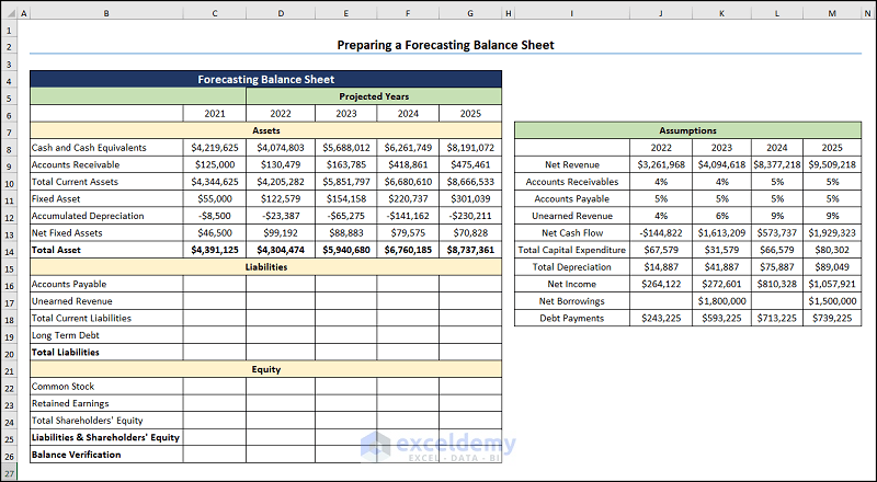
• Lastly, use the Fill Handle Tool to copy the formula across the cells.

Now, the output should look like the picture given below.

Read More: How to Make Projected Balance Sheet in Excel (with Quick Steps)

Similar Readings

• How to Make Stock Balance Sheet in Excel (with Quick Steps)
• Balance Sheet Format in Excel with Formulas (Create with Easy Steps)
• Create a Balance Sheet Format for Trading Company in Excel
• How to Create NGO Balance Sheet Format in Excel (4 Easy Steps)
• Balance Sheet Format of a Company in Excel (Download Free Template)

📌 Step 2: Compute the Liabilities

• Third, navigate to the C16 and C17 cells >> enter the Accounts Payable and the Unearned Revenue >> proceed to the C10 cell and obtain the Total Current Liabilities

Here, C16 and C17 cells refer to the values of $65,000 and $336,125.

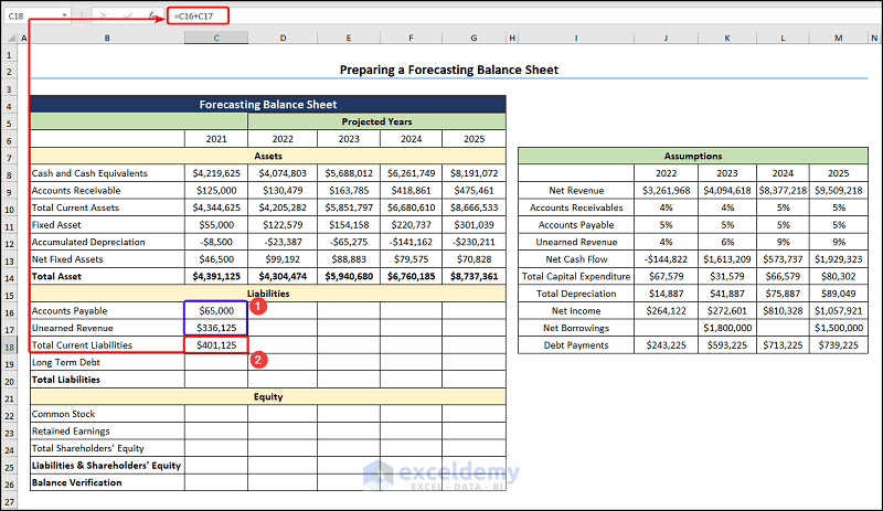
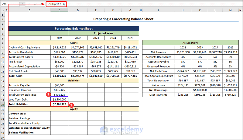
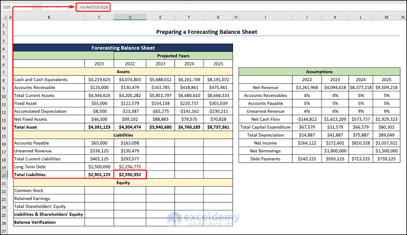
• Now, type in the Long Term Debt in the C19 cell >> calculate the Total Liabilities amounting to $2,901,125.

In the above expression, C18 and C19 cells represent the Total Current Liabilities ($401,125) and the Long Term Debt ($2,500,000).

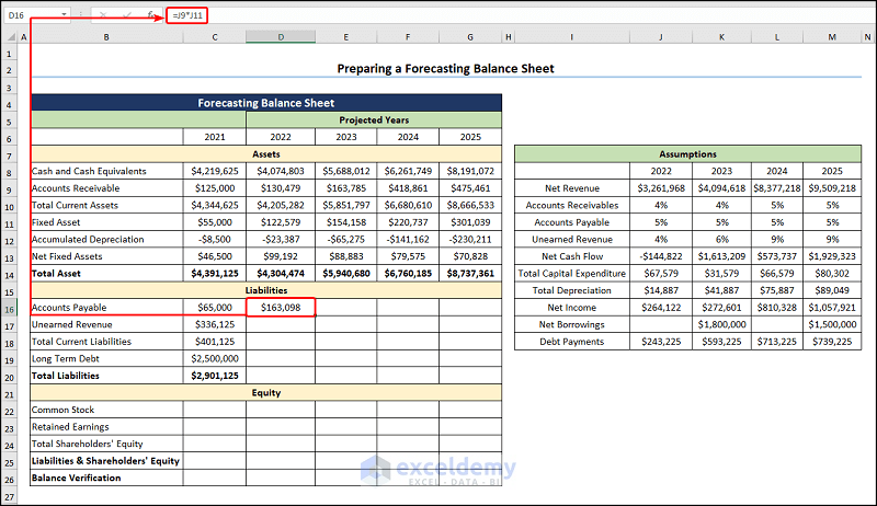
• Fourth, move to the D16 cell >> calculate the Accounts Payable for 2022.

In this formula, the J9 and J11 cells represent the Net Revenue ($3,261,968) and the Account Payable (5%) respectively.

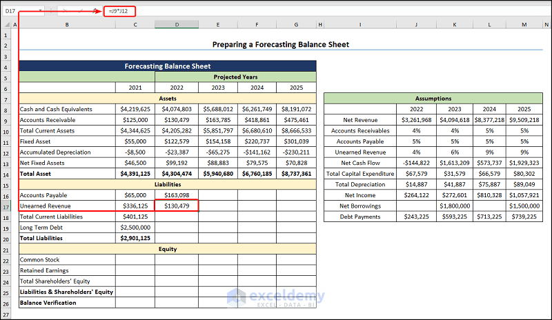
• In a similar style, obtain the Unearned Revenue with the formula given below.

Here, the J9 and J12 cells represent the Net Revenue ($3,261,968) and the Unearned Revenue (4%) respectively.

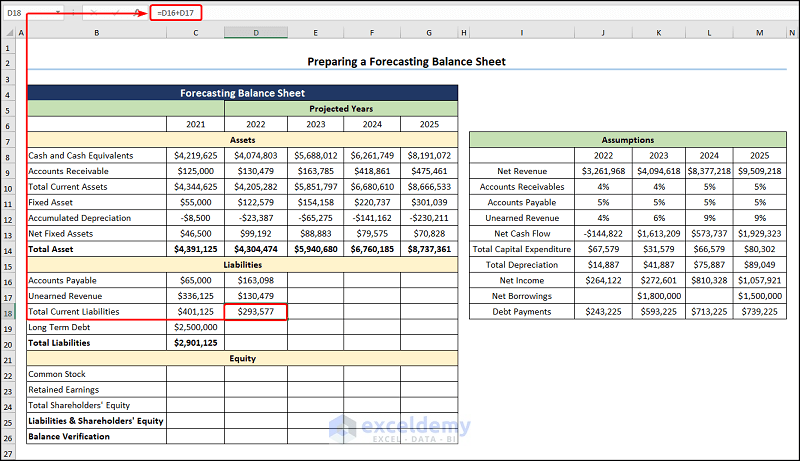
• Next, jump to the D18 cell to get the Total Current Liabilities with a value of $293,577.

In this expression, the D16 and D17 cells point to the Accounts Payable ($163,098) and Unearned Revenue ($130,479).

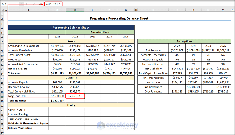
• In turn, obtain the Long Term Debt which amounts to $2,256,775.

In the above equation, the C19, J17, and J18 cells refer to the Long Term Debt for 2021 ($2,500,000), Net Borrowings ($0), and Debt Repayments for 2022 ($243,225).

• Finally, compute the Total Liabilities with the given expression >> drag the formula across the other cells.

Here, the D18 and D19 cells represent the Total Current Liabilities and the Long Term Debt respectively.

Read More: How to Create Vertical Balance Sheet Format in Excel

📌 Step 3: Calculate the Equity

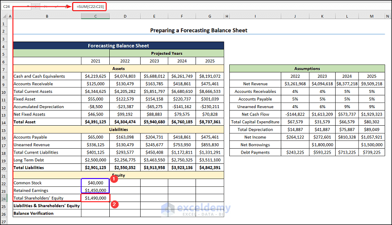
• Fifth, proceed to the C22 and C23 cells >> enter the amounts for the Common Stock ($40,000) and Retained Earnings ($1,450,000).
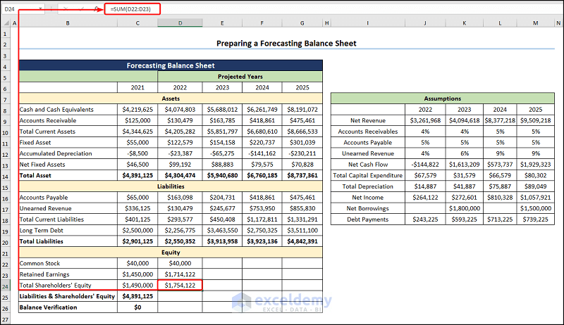
• Now, obtain the Total Shareholder’s Equity using the formula below.

Here, C22 and C23 cells indicate the Common Stock and Retained Earnings.

• Following this, add the Total Liabilities and the Total Shareholder’s Equity.

In this formula, C20 and C24 cells represent the Total Liabilities ($2,901,125) and the Total Shareholder’s Equity ($1,490,000) respectively.

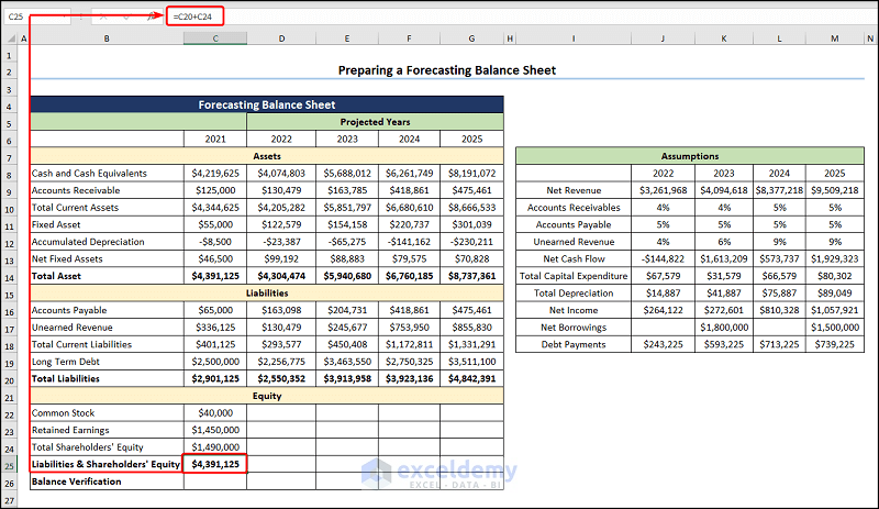
Consequently, the Balance Verification becomes zero, which satisfies the equation: Asset = Liability + Equity

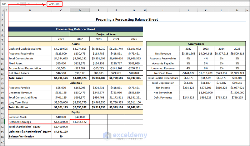
• Lastly, calculate 2022 Retained Earnings using the expression below.

In this case, the C23 cell refers to the 2021 Retained Earnings ($1,450,000) whereas the J16 cell points to the assumed Net Income of $264,122.

• Additionally, calculate the Total Shareholder’s Equity.

In this expression, D22 and D23 cells represent the Common Stock and Retained Earnings.

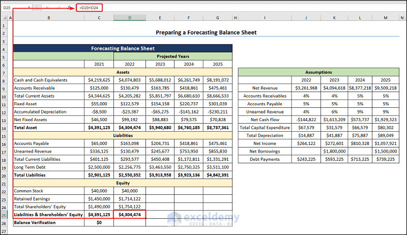
• In turn, compute the Liabilities and Shareholder’s Equity and copy the formula across the other cells.

Here, D20 and D24 cells point to the Total Liabilities and Total Shareholder’s Equity.

Finally, your results should look like the screenshot given below.

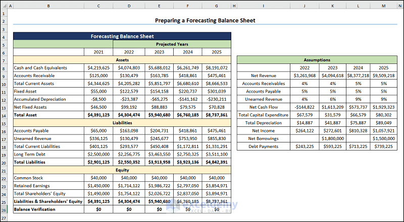
Admittedly, I have skipped the process of making Excel Format for Projected Financial Statements. You may explore it if you wish.

Read More: How to Create Common Size Balance Sheet in Excel

Practice Section

In the end, we’ve provided a Practice section on the right side of each sheet so you can practice yourself.

Conclusion

Henceforth, I have shown you how to make a forecasting balance sheet in Excel. So, I suggest you read the full article carefully and apply the knowledge to your needs. Moreover, you can also download our free workbook to practice. On the whole, I hope you find this article helpful and informative. Moreover, if you have any further queries or recommendations, please feel free to comment and visit ExcelDemy for many more articles like this.

Related Articles

• Create Projected Balance Sheet Format for Bank Loan in Excel
• Perform Balance Sheet Ratio Analysis in Excel
• How to Make Balance Sheet Format in Excel for Individual
• Schedule 6 Balance Sheet Format in Excel
• How to Prepare Balance Sheet from Trial Balance in Excel
• Balance Sheet Format in Excel for Proprietorship Business
• Income and Expenditure Account and Balance Sheet Format in Excel