What Is a Projected Balance Sheet?
A projected balance sheet, also called a pro forma balance sheet, contains all the financial information (such as assets, liabilities and owner’s equity) of an organization. A projected balance sheet always satisfies the following equation:
Total Assets = Total Liabilities + Total EquityIn the equation,
Total Assets: refers to the sum of the resources that a company or organization owns, such as cash, inventories, prepaid expenses, accounts receivable, licenses, etc.
Total Liabilities: is the sum of all the organization’s debt, such as accounts payable, unearned revenue, mortgage payable, etc.
Total Equity: is the net worth of an owner’s investment in a company after deducting all liabilities.
Method 1 – Manually Creating Projected Balance Sheet Format for 3 Years
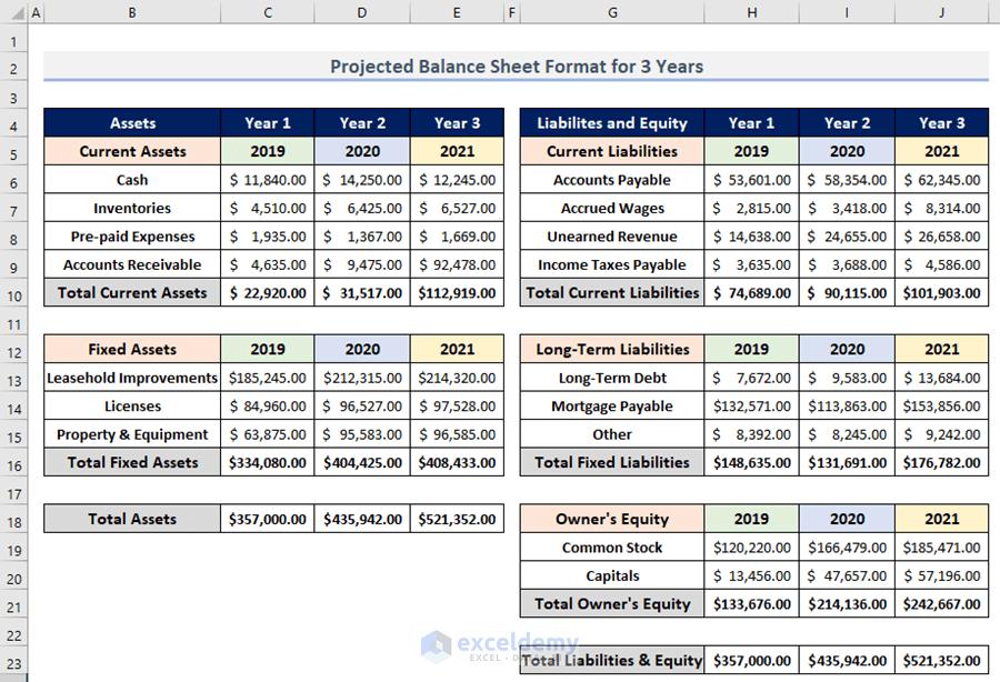
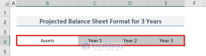
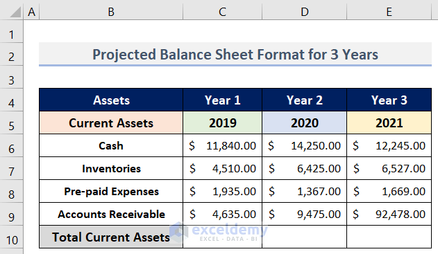
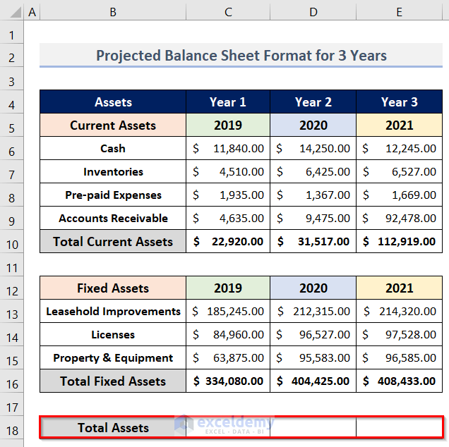
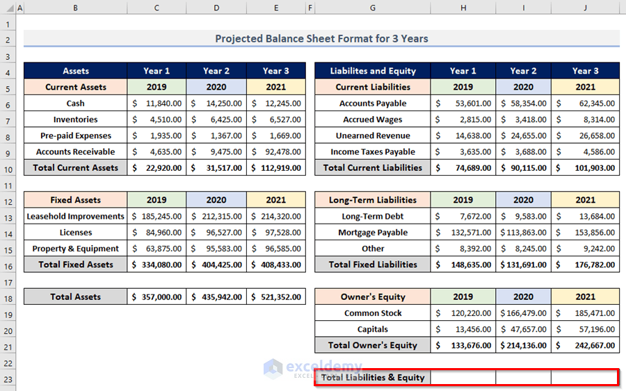
Here, Year 1 is 2019, Year 2 is 2020, and Year 3 denotes 2021. We will create a projected balance sheet like the following picture.
Step 1 – Creating Dataset of Current Assets
- Open a worksheet in Excel.
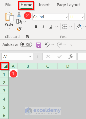
- Select the entire worksheet with a left-click on the triangle located at the top-left corner of the worksheet.
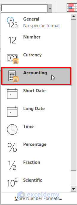
- Go to the Home tab.
- Click on the Number Format drop-down in the Number group.
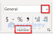
- Select Accounting from the dropdown menu.
A dollar sign ($) will now be appended to any value in the worksheet.
- Enter Assets, Year 1, Year 2 & Year 3 in the range B4:E4.
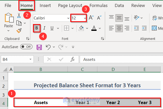
- Select range B4:E4.
- Go to the Home tab.
- Change the Font Size to 12.
- Click on B (for Bold).
- Change the Fill Color (to Dark Blue).
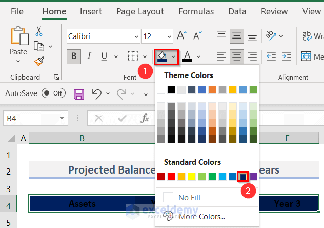
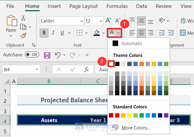
- Select the font color (White) by clicking on the Font Color dropdown.
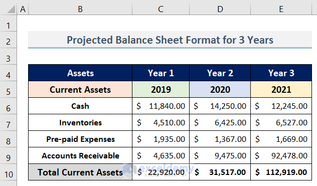
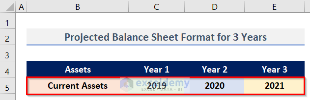
- Create headings (B5:E5) for the Current Assets table as in the image below.
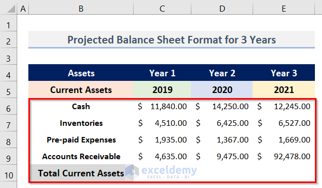
- Enter the names of the Current Assets and Total Current Assets in the B6:B10 range.
- Enter the asset values for the 3 years in the C6:E9 range.
- Select the B4:E10 range.
- Go to the Home tab.
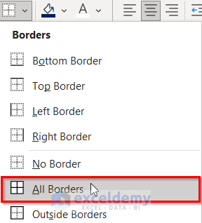
- Click on the Border dropdown from the Font group.
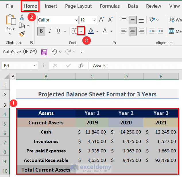
- Select All Borders from the dropdown menu.
The table (B4:E10) will look like the following image.
- To calculate the Total Current Assets of Year 1, enter the formula below in cell C10:
=SUM(C6:C9)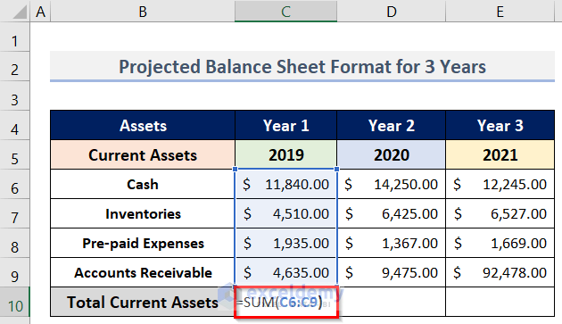
- Press Enter.
The Total Current Assets for Year 1 are returned.

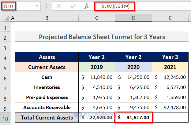
- In the same way, add the Currents Assets of Year 2 by entering the following formula in cell D10:
=SUM(D6:D9)- Press the Enter key to get the result in cell D10.
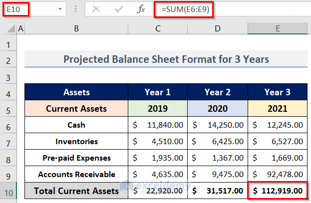
- Add the Total Current Assets for Year 3 by entering the following formula in cell E10:
=SUM(E6:E9)- Press Enter to return the result.
Step 2 – Estimating Total Fixed Assets
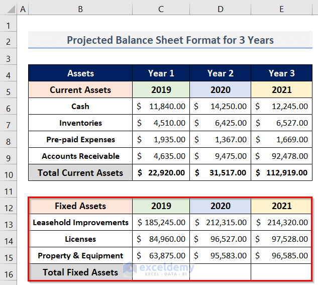
- Create a dataset (B12:E16) of Fixed Assets for the 3 years by following the process shown in the previous step.
- To sum the values of Fixed Assets in Year 1, enter the formula below in cell C16:
=SUM(C13:C15)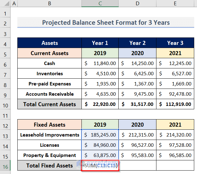
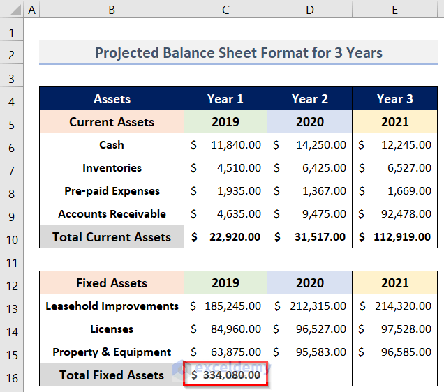
- Press Enter to return the result.
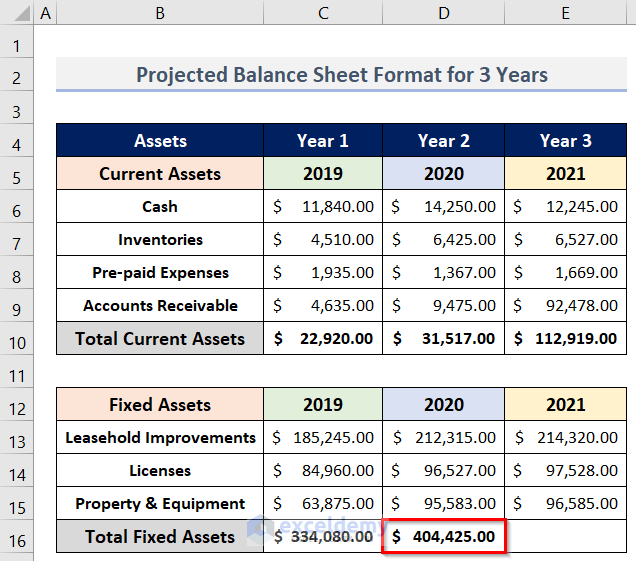
- To add the Fixed Assets in Year 2, enter the following formula in cell D16:
=SUM(D13:D15)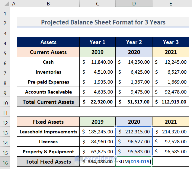
- Press Enter to return the result.
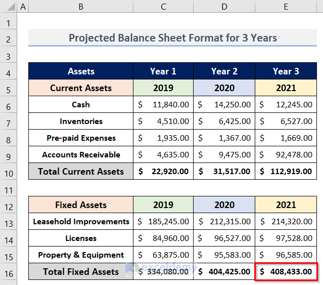
- To find the Total Fixed Assets in Year 3, enter the formula below in cell E16:
=SUM(E13:E15)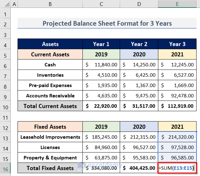
- Press Enter to return the result.
Read More: Balance Sheet Format for Construction Company in Excel
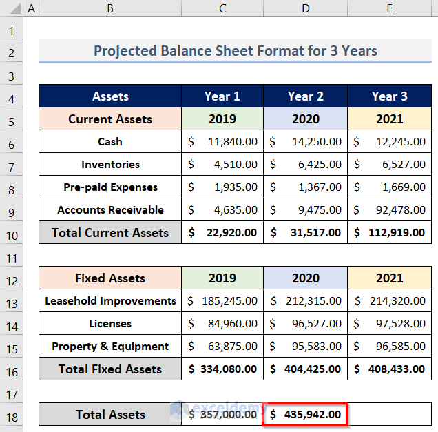
Step 3 – Finding Total Assets
To determine the Total Assets, simply add the Total Current & Fixed Assets.
- Create a row (B18:E18) for storing the Total Assets values for the 3 years.
- In cell C18, enter the following formula:
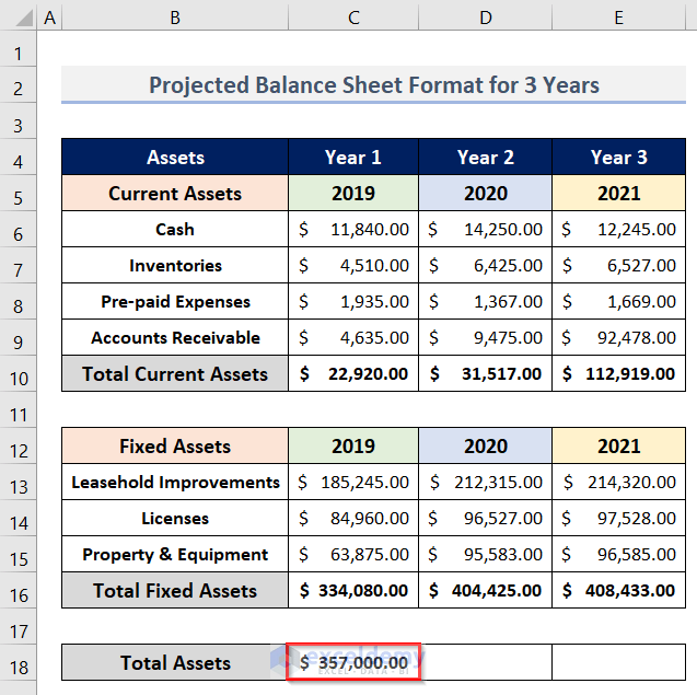
=SUM(C10,C16)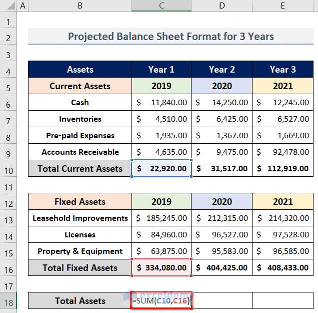
- Press Enter to return the result.
- In cell D18, to calculate the Total Assets in Year 2, enter the following formula:
=SUM(D10,D16)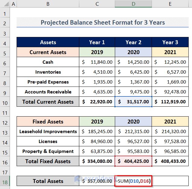
- Press Enter to return the result.
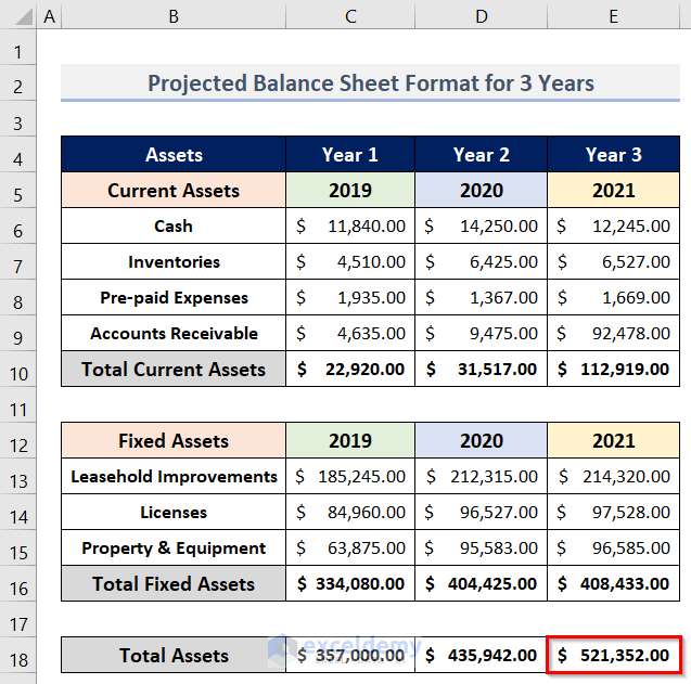
- To determine the Total Assets in Year 3, enter the following formula in cell E18:
=SUM(E10,E16)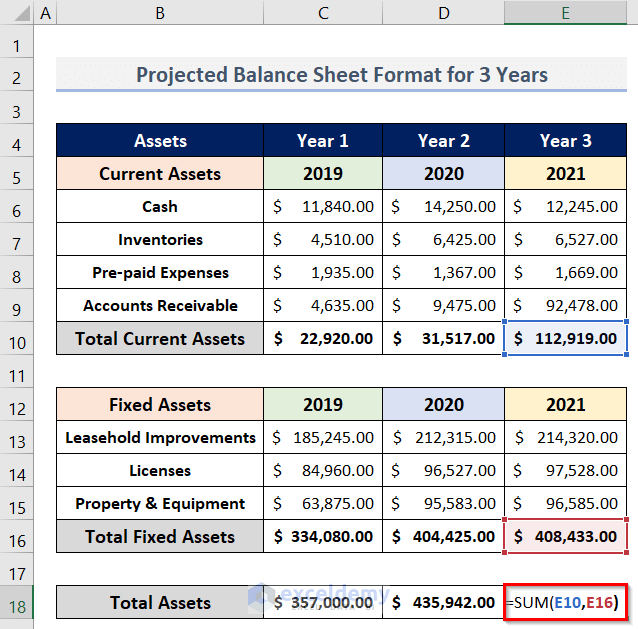
- Press Enter to return the result.
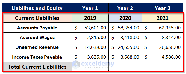
Step 4 – Making Dataset of Current Liabilities
- Insert headings (G4:J4) for Liabilities and Equity of Year 1, Year 2, and Year 3 by following the process in Step 1.

- Create a table for the Current Liabilities for the three years (as in Step 1).
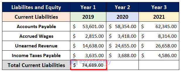
- To find the Total Current Liabilities of Year 1, enter the following formula in cell H10:
=SUM(H6:H9)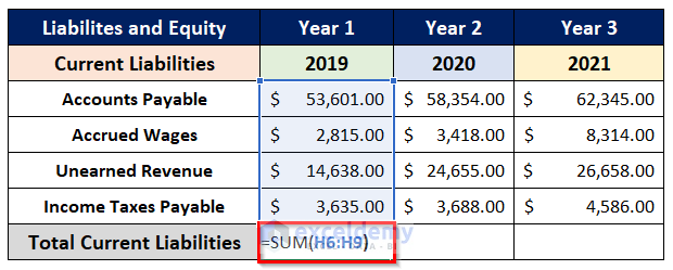
- Press Enter to return the result.
- To find the Total Current Liabilities in Year 2, enter the formula below in cell I10:
=SUM(I6:I9)- And for Year 3, enter the following formula in cell J10:
=SUM(J6:J9)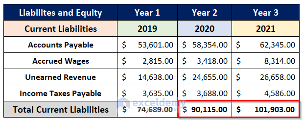
Read More: Create a Balance Sheet Format for Trading Company in Excel
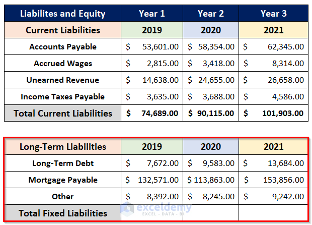
Step 5 – Determining Total Long-Term Liabilities
- Create a dataset (G12:J16) for the Long-Term Liabilities.
The dataset will look like the following image.
- In cell H16, to add the Fixed or Long-Term Liabilities for 2019, enter the following formula:
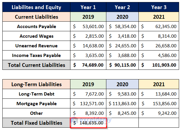
=SUM(H13:H15)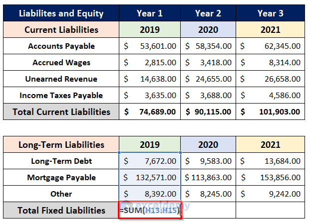
- Press Enter to return the result.
The output is returned ($ 148,635.00).
In the same way, estimate Total Fixed Liabilities for 2020 and 2021 respectively.
- For the year 2020, use the formula below in cell I16:
=SUM(I13:I15)- Similarly, for 2021, use the following formula in cell J16:
=SUM(J13:J15)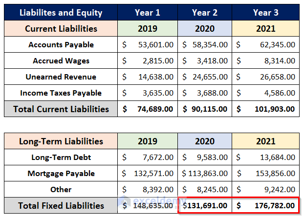
Step 6 – Calculating Total Owner’s Equity
- Prepare a table (G18:J21) by entering the names and values of the Owner’s Equity.
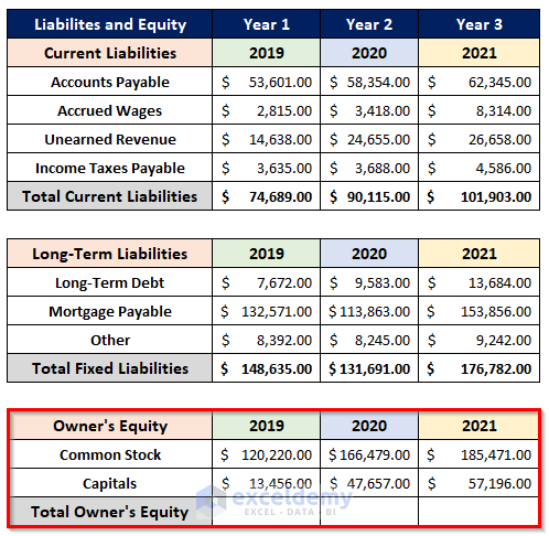
- To calculate the Total Owner’s Equity for Year 1, enter the formula below in cell H21:
=SUM(H19:H20)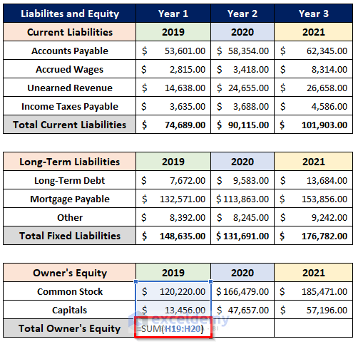
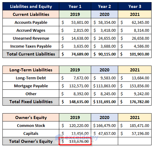
- Press Enter.
The result ($133,676.00) is returned in cell H21.
- For Year 2, enter the formula below in cell I21:
=SUM(I19:I20)- And for Year 3, enter the following formula in cell J21:
=SUM(J19:J20)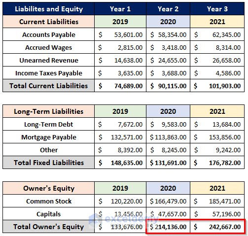
Read More: Balance Sheet Format of a Company in Excel
Step 7 – Adding Total Current & Fixed Liabilities with Total Equity
We will perform this calculation in the H23:J23 range.
- To calculate Total Liabilities & Equity in 2019, enter the following formula in cell H23:
=SUM(H10,H16,H21)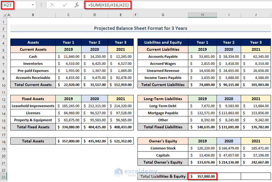
- For 2020, enter the formula below in cell I23:
=SUM(I10,I16,I21)- And for 2021, enter the following formula in cell J23:
=SUM(J10,J16,J21)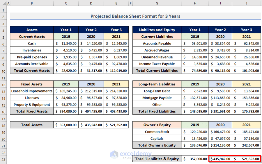
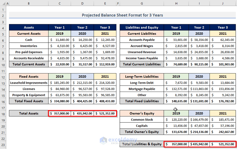
Final Output
We have a complete projected balance sheet format in Excel for 3 years.
In this balance sheet, the Total Assets (C18:E18) and Total Liabilities & Equity (H23:J23) are equal in each of the 3 years.
Read More: Income and Expenditure Account and Balance Sheet Format in Excel
Method 2 – Using Excel Templates to Make a Projected Balance Sheet Format for 3 Years
Microsoft Excel contains some built-in balance sheet templates that we can easily modify as per our requirements.
Steps:
- Go to the File tab.
- Select the New option.
- Type ‘Balance Sheet’ in the search box.
- Click on the search icon.
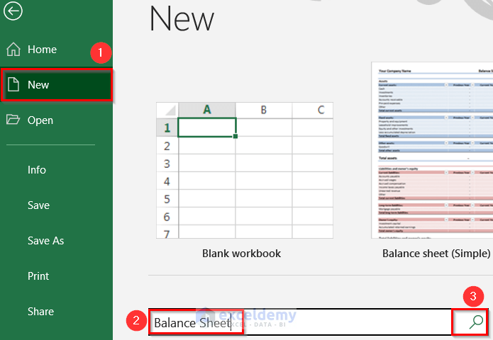
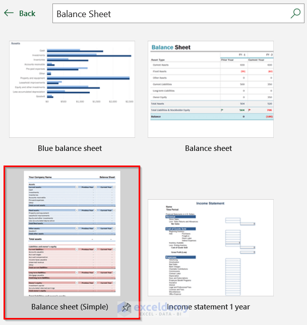
Some Balance Sheet templates will appear.
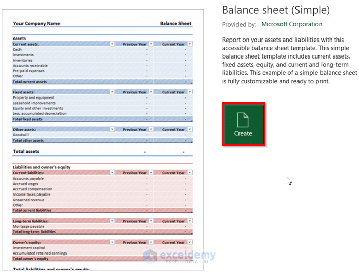
- Select an option. In our case, we selected the Balance Sheet (Simple) as it looks close to the one we require.
- Click on the Create button.
A new Excel workbook will open containing 3 worksheets.
- Select Balance Sheet from the sheet tab section.
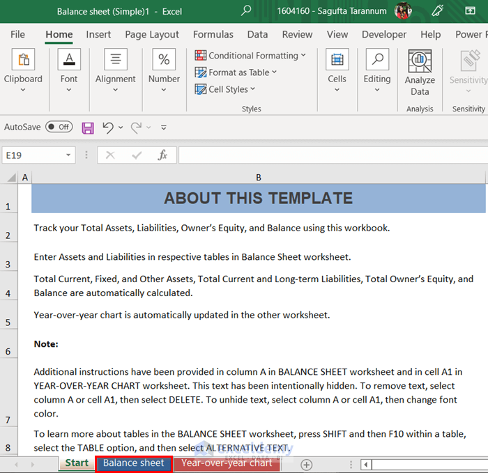
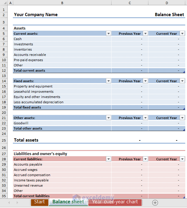
The Balance Sheet will appear.
- Modify this Balance Sheet as desired.
In our case, we need a balance sheet for three years, but this balance sheet is only for two years.
- Add another column.
Read More: How to Create Daily Bank Balance Report Format in Excel
Things to Keep in Mind
- In the balance sheet, the Total Assets, Total Liabilities, and Equity have to be equal in all years.
- Before any depreciation value, always use a minus (–) symbol.
Download Practice Workbook
Related Articles
- Balance Sheet Format in Excel for Proprietorship Business
- Create a Format of Balance Sheet of Partnership Firm in Excel
- Create Projected Balance Sheet Format for Bank Loan in Excel
- How to Create NGO Balance Sheet Format in Excel
<< Go Back to Balance Sheet | Finance Template | Excel Templates
Get FREE Advanced Excel Exercises with Solutions!
