To know the financial stability of a company or organization, we use the Balance Sheet. We can apply different Excel formulas and different features to create it. In this article, we are going to create a Horizontal Balance Sheet Format in Excel with some easy steps.
What Is a Balance Sheet?
In the accounting of a business, there are three core financial statements. One is the Balance Sheet and the other two are the Income Statement & Cash Flow Statement.
A balance sheet summarizes the financial amounts. It is used to measure the financial strengths and weaknesses as well as the profit or loss of a company or organization.
Balance Sheet Structure in Excel
A balance sheet has three essential parts. They are; Assets, Liability & Equity. Combined they can be written as:
Assets are the sources that cause benefits in the future. They are land, cash, equivalents of cash, equipment, buildings, patents, goodwill, etc.
The things that a company’s debts or financial obligations to a person or an organization are known as Liabilities. They are bank loans, mortgages, payable income tax, etc.
The net assets or capital of the owner or shareholders after all the liabilities are paid off is known as Equity. A company’s shareholders can distribute the value among them when sold.
Step by Step Procedures to Create Horizontal Balance Sheet Format in Excel
In the Horizontal Balance Sheet, the Assets, Liabilities & Equity columns are shown in an Excel table where we can see the assets on the left side of the table.
On the other hand, the liabilities & equity parts are seen on the right side of the table.
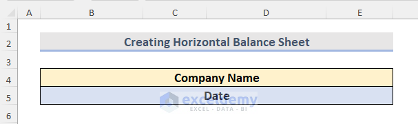
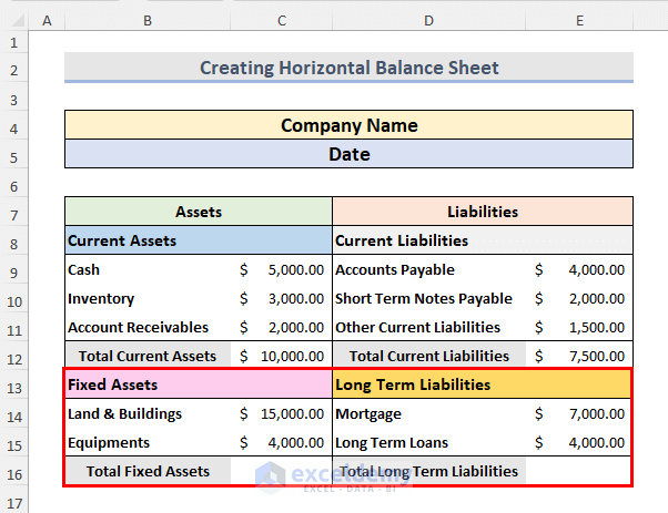
Step 1: Create a Horizontal Balance Sheet Heading
- First, insert the Company Name in row 4.
- Then the Date in row 5.
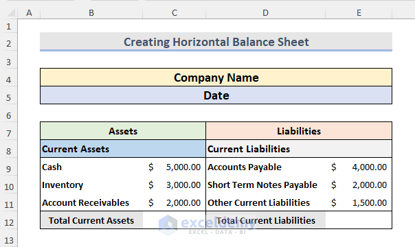
Step 2: Input Current Assets & Current Liabilities Data
- Now we will enter the Current Assets (Cash, Inventory, Account Receivable) in range B9:C11.
- After that, in range D9:D11, we will enter the Current Liabilities (Account Payable, Short Term Notes Payable, Other Current Liabilities).
- We will also calculate the Total Current Assets & Total Current Liabilities in cells C12 & E12 respectively.
Note: We need to make the number column into Accounting. To do that,
Press Ctrl + 1 to open the Format Cells dialogue box > Choose Accounting from the Category list > Press OK.
Read More: How to Create Tally Debit Note Format in Excel
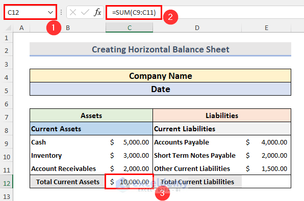
Step 3: Calculate Total Current Assets and Total Current Liabilities
- Next, select the cell C12 and write the formula below:
=SUM(C9:C11)- Hit Enter to see the Total Current Assets result.
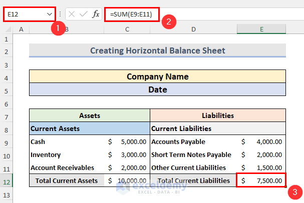
- Further, in cell E12, write down the below formula:
=SUM(E9:E11)- Press the Enter button.
- As a result, we will see the Total Current Liabilities.
Step 4: Insert Fixed Assets & Long-Term Liabilities Data
- At this moment, enter the Fixed Assets (Land & Buildings, Equipments) & Long Term Liabilities (Mortgage, Long Term Loans) data in range B14:C15 & D14:E15 respectively.
Read More: Revised Schedule 3 Balance Sheet Format in Excel with Formula
Step 5: Estimate Total Fixed Assets & Total Long Term Liabilities Data
- Then to estimate the Total Fixed Assets, select the cell C16.
- Write the formula below and hit Enter to see the result.
=SUM(C14:C15)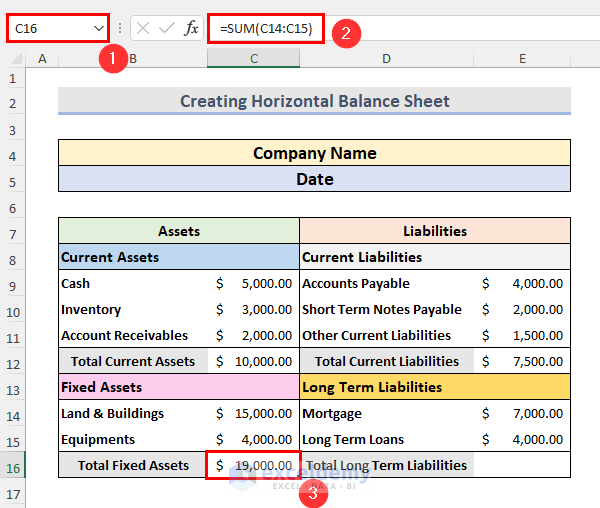
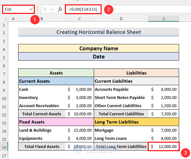
- Again for Total Long Term Liabilities, insert the below formula at cell E16:
=SUM(E14:E15)- After that, hit the Enter button on the keyboard.
Read More: Balance Sheet Format in Excel with Formulas
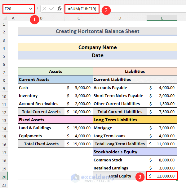
Step 6: Add Stockholder’s Equity Data & Calculate Total Equity
- In the end, we need to add the Stockholder’s Equity data (Common Stock, Retained data) in the range D18:E19.
- Now in cell E20, insert the below formula and press Enter:
=SUM(E18:E19)- Here, we will see the Total Equity value.
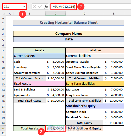
Step 7: Estimate Total Assets, Liabilities & Equity
- Finally, we are going to estimate Total Assets, Liabilities & Equity.
- First, select cell C21.
- Write down the formula below:
=SUM(C12,C16)- Further, press Enter.
- Consequently, we will see the Total Assets value.
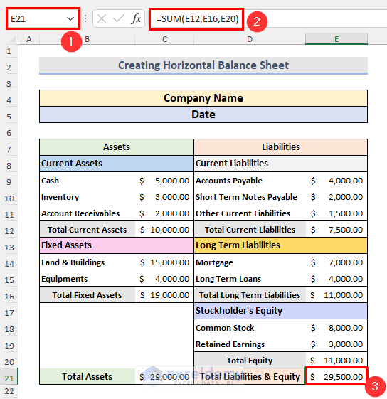
- Now select cell E21.
- Insert the below formula and hit Enter.
=SUM(E12,E16,E20)- In the end, we will see the Total Liabilities & Equity value.
Read More: Schedule 6 Balance Sheet Format in Excel
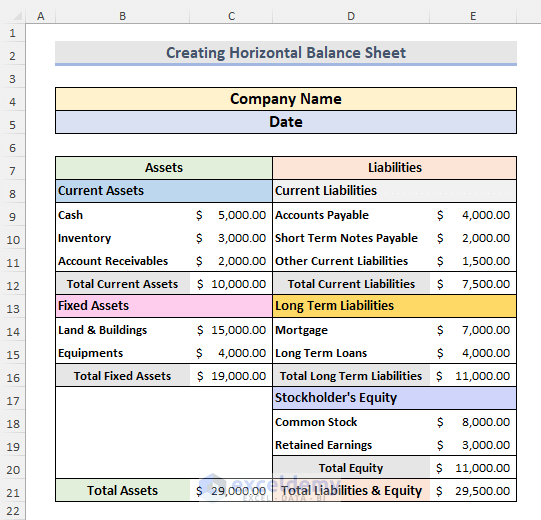
Final Output
Our final Horizontal Balance Sheet will look like the below screenshot.
Things to Remember
- It can be used in Banks for business loan purposes.
- We can easily monitor the financial position, which means a company’s loss or profit rate.
- We cannot include the assets in the calculation which are under development.
- It helps us to make a proper future business plan based on its financial statements.
Download Practice Workbook
Download the practice workbook from here.
Conclusion
Following these steps, we can quickly create a horizontal balance sheet in Excel. There is a practice workbook that we added. Go ahead and give it a try. Feel free to ask anything or suggest any new methods.
Related Articles
- How to Create Vertical Balance Sheet Format in Excel
- How to Make Hotel Balance Sheet Format in Excel
- How to Perform Balance Sheet Ratio Analysis in Excel
- How to Add Balance Sheet Graph in Excel
<< Go Back to Balance Sheet | Finance Template | Excel Templates
Get FREE Advanced Excel Exercises with Solutions!
