Revised Schedule 3 Balance Sheet Format in Excel with Formula

In this article, we will show you quick steps on how to create a revised Schedule 3 balance sheet format in Excel with a formula.


Balance Sheet

It summarizes the financial position of the company after a certain period and is also known as a Statement of Financial Position/condition. In general, a balance sheet consists of three parts. And, these are assets, liabilities, and owners’ equity. A balance sheet provides a glimpse of the company’s finances. The balance sheet consists of the company’s liabilities, assets, and owner’s equity. Balance sheets are organized according to the equation:

Assets = Liabilities + Owner’s Equity

  • Assets: These are the main resources owned by the company. Assets can be categorized into many types. Examples- current and fixed assets, tangible and intangible assets, etc.
  • Liabilities: They are things that the company owes to a person or another company, like cash, loans, etc.
  • Owner’s Equity: It represents the value for a company’s shareholders after all the company’s assets have been sold off and all company liabilities have been paid off.

Revised Schedule 3 Balance Sheet

Indian company law is governed by the 2013 Companies Act, an Act of the Indian Parliament. The incorporation of a company, the duties of a company, the election of directors, and the dissolution of a company are all governed by this document. Schedule III, or 3 is a part of that act. This represents the “general instructions for the preparation of the balance sheet and income statement of a company.” There are three divisions of companies:

  • Division I → This is for the companies that need to maintain the “companies rules (accounting standards) 2006”
  • Division II → This is for the companies that must adhere to the “companies rules (Indian accounting standards) 2015”
  • Division III → For the non-banking financial institutions following the “companies rules  (Indian accounting standards) 2015”

The 2021 amendment to this schedule emphasizes the need for companies to disclose more information. On the basis of this modification, we’ll demonstrate how to make a revised Schedule 3 balance sheet format in Excel with a formula.


Step-by-Step Procedures to Create Revised Schedule 3 Balance Sheet Format In Excel with Formula

There will be 3 simple steps to show you the procedures to create a revised Schedule 3 balance sheet format in Excel with the formula. We will set up the balance sheet format in the first step. After that, we will input the note details in the second step. Lastly, we will link the values from the notes to the balance sheet format.


Step 1: Setting Up Balance Sheet Format

In this first step, we will specify the balance sheet format according to the revised Schedule 3 in Excel with the formula. Our company name is “ABC Company Limited,” and this is a Division I company. We are creating the balance sheet for March 31, 2022, as the Indian fiscal year starts on April 1.

  • Firstly, type the following fields on the spreadsheet.
  • Secondly, add the note numbers which we will input in the second step.
  • Moreover, we will add two columns for this year and the last year.
  • So, in the following image, you can see the equity and liabilities part of the balance sheet.
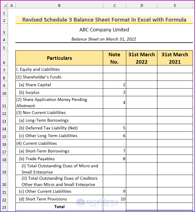
Setting Up Balance Sheet Format to Create Revised Schedule 3 Balance Sheet Format in Excel with Formula

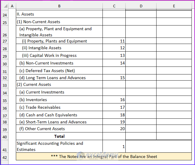
  • Lastly, you can observe the assets part of the balance sheet.
  • Thus, we completed the first step of creating the basic format for the revised Schedule 3 balance sheet.

Read More: How to Create Tally Debit Note Format in Excel


Step 2: Entering Note Details

We will input the values inside the notes and then link those values to the respective cells from the balance sheet format in this step. There are twenty notes for the revised Schedule 3 balance sheet format. The first note is for the company’s accounting policies. Then, the next nine notes are for the equity and liability parts. Finally, the last 10 notes are for the assets part of the balance sheet.

  • To begin with, type the company accounting policies in the “note 1” sheet.
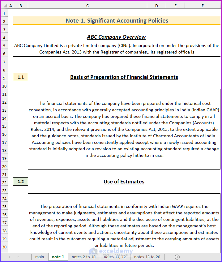
Entering Note Details to Create Revised Schedule 3 Balance Sheet Format in Excel with Formula

  • After that, type the details of note 2 for the equity share capital. Here the values are inserted randomly.
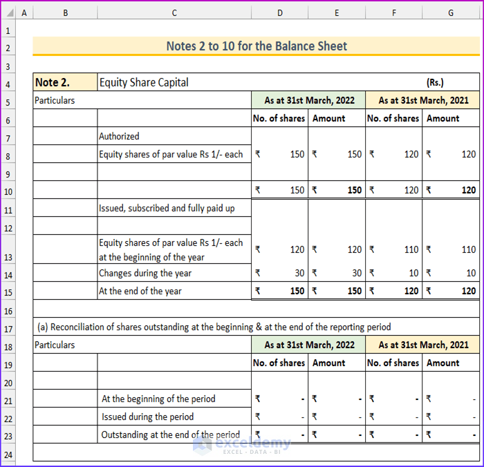
  • Next, type the details of note 3 for the surplus.
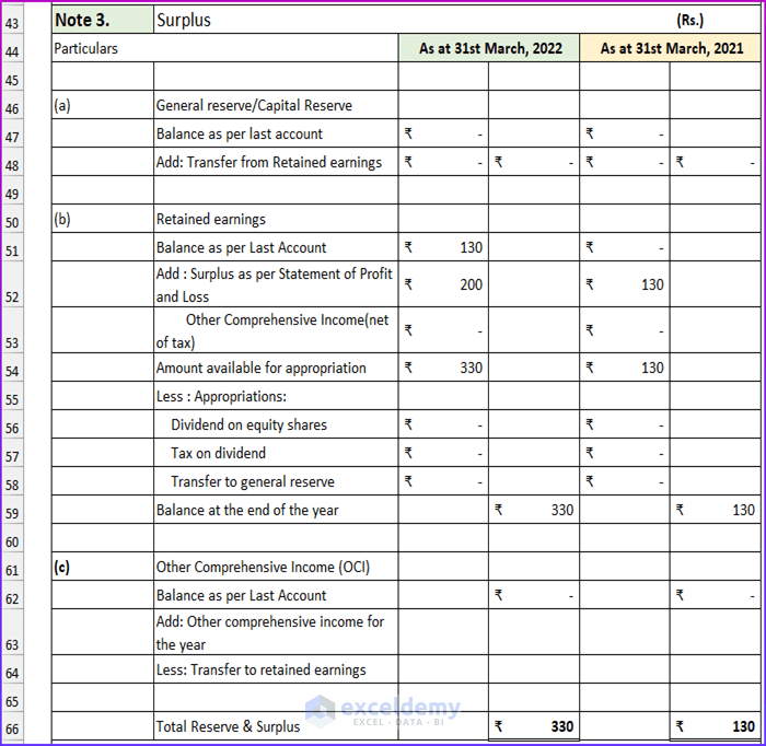
Note 3 to Create Revised Schedule 3 Balance Sheet Format in Excel with Formula

  • Then, type the details of the share application money pending allotments.

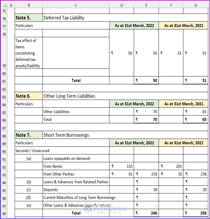
  • Next, type the values for notes 5, 6, and 7.

Notes 5,6,7 to Create Revised Schedule 3 Balance Sheet Format in Excel with Formula

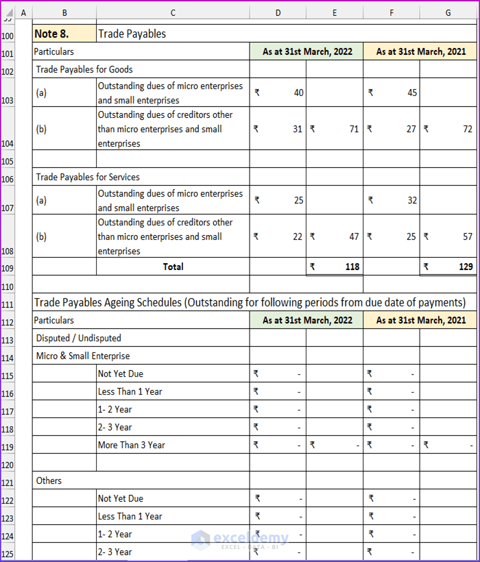
  • After that, type the details for note 8.

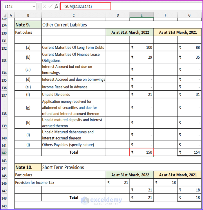
  • Afterward, type the following formula to find the total values of other current liabilities. Moreover, type the details for note 10.

=SUM(E132:E141)

Notes 9,10 to Create Revised Schedule 3 Balance Sheet Format in Excel with Formula

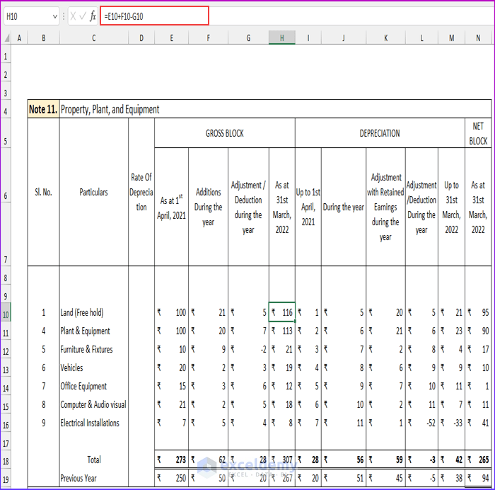
  • Then, type the following formula to find the value of the total gross block.

=E10+F10-G10

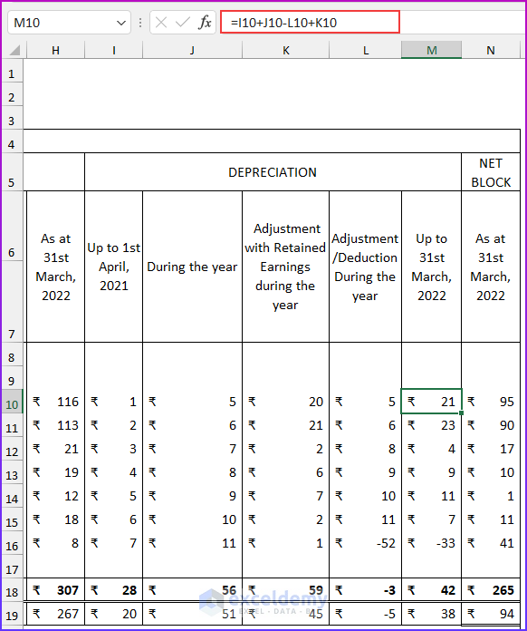
  • Next, type this formula to calculate the value of depreciation.

=I10+J10-L10+K10

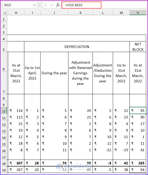
  • After that, type this formula to find the value of the netblock.

=H10-M10

  • Next, type the following formula to return the total amount. Additionally, type the previous year’s values.

=SUM(G10:G16)
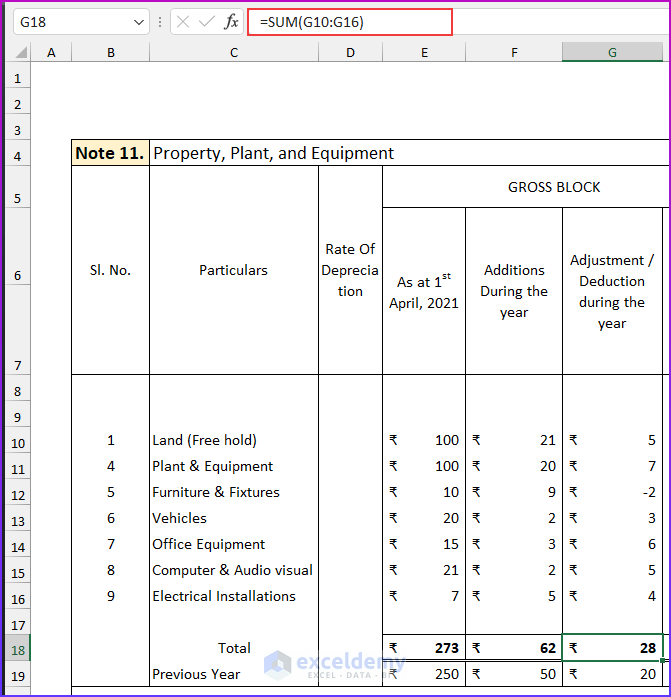
Note 11 to Create Revised Schedule 3 Balance Sheet Format in Excel with Formula

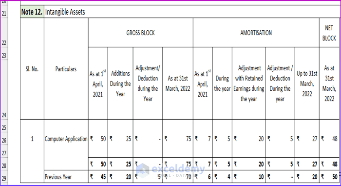
  • After that, type the details for note 12.

  • Then, type the following values to complete note 13.
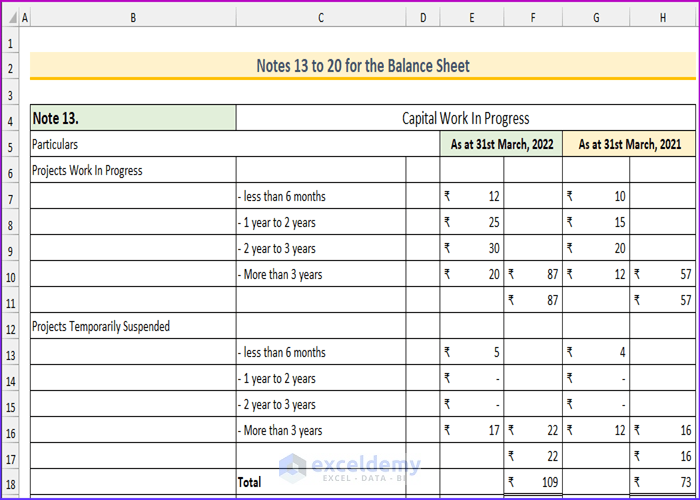
Note 13 to Create Revised Schedule 3 Balance Sheet Format in Excel with Formula

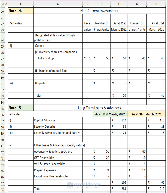
  • Then, type the details for notes 14 and 15.

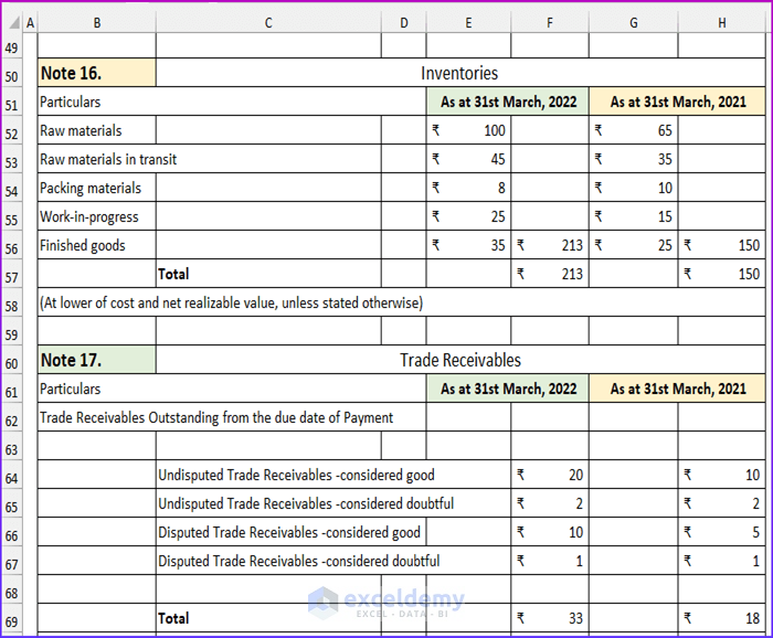
  • Then, type these values to complete notes 16 and 17.

Note 16,17 to Create Revised Schedule 3 Balance Sheet Format in Excel with Formula

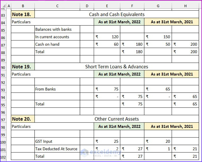
  • Lastly, type the following values. Consequently, this will complete the notes for the revised Schedule 3 balance sheet format in Excel.

Read More: Balance Sheet Format in Excel with Formulas


Step 3: Linking Notes to Balance Sheet

In this last step, we will link to the values from the notes on the balance sheet. We will use the SUM function to calculate the total values. Without further ado, let us see how we can complete the process.

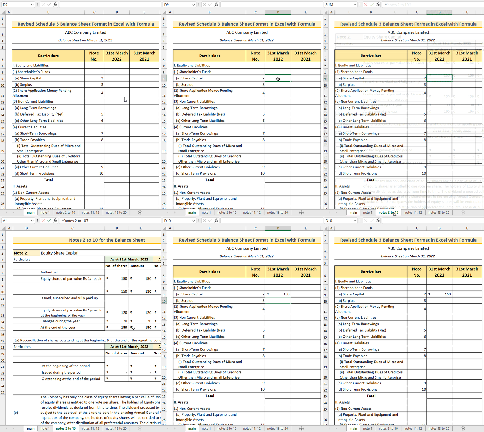
  • Firstly, link the values for the share capital from the “notes 2 to 10” sheet. In the formula bar, we can see the following formula.

='notes 2 to 10'!E15

Linking Notes to Create Revised Schedule 3 Balance Sheet Format in Excel with Formula

  • Secondly, link the values from the notes to the rest of the values in the balance sheet.
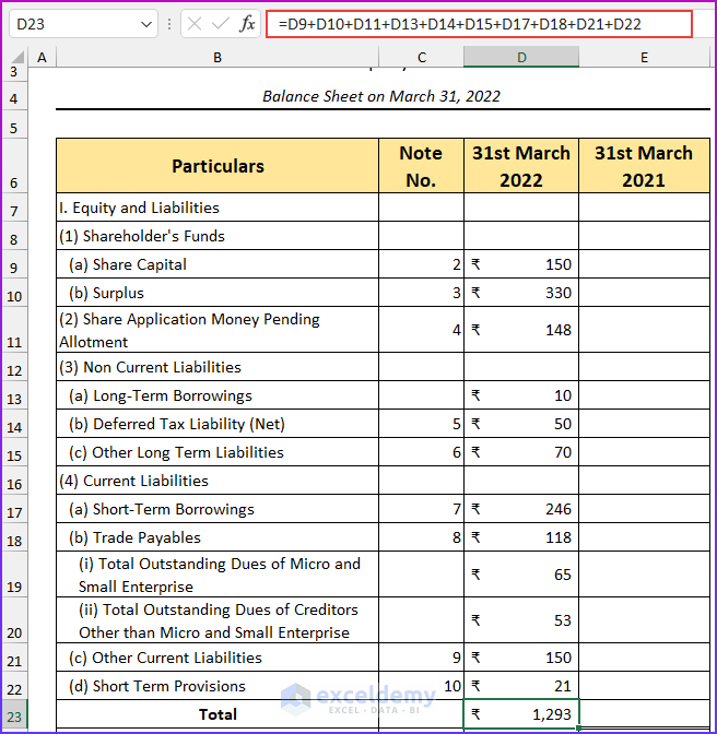
  • Thirdly, type the following formula in cell D23 to find the total values of equity and liability.

=D9+D10+D11+D13+D14+D15+D17+D18+D21+D22
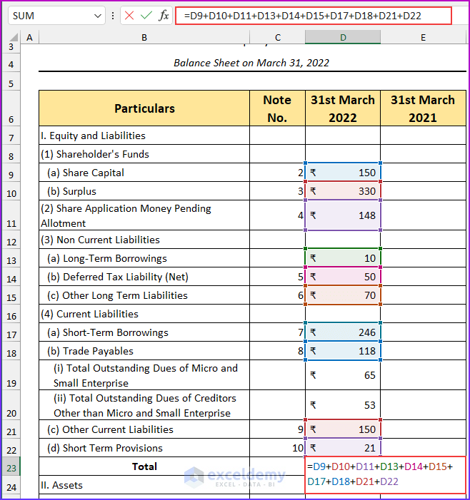
  • Then, press ENTER and it will return the total value.

Total Equity and Liability to Create Revised Schedule 3 Balance Sheet Format in Excel with Formula

  • Afterward, type this formula in cell D40 to calculate the value of the total assets.

=SUM(D27:D39)
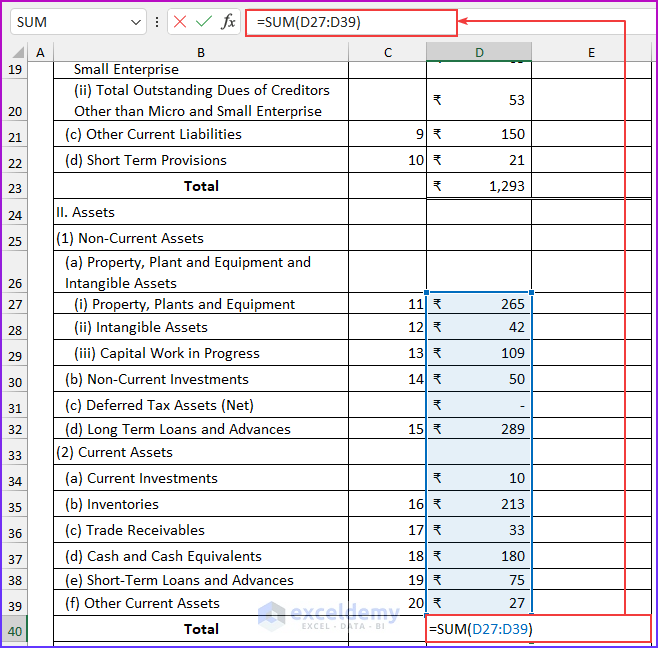
  • Lastly, press ENTER and we can see that the balance sheet balances.
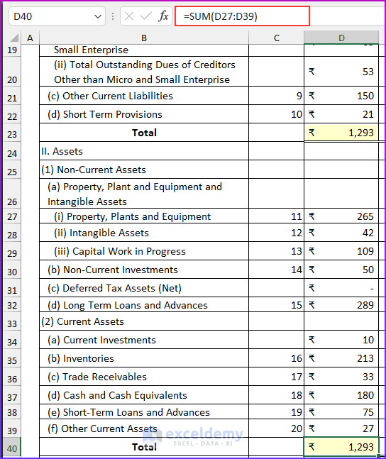
Total Assets to Create Revised Schedule 3 Balance Sheet Format in Excel with Formula

  • Lastly, complete the values for the year 2021 and the final output will look similar to this snapshot. Here, we have hidden some rows for better visualization.
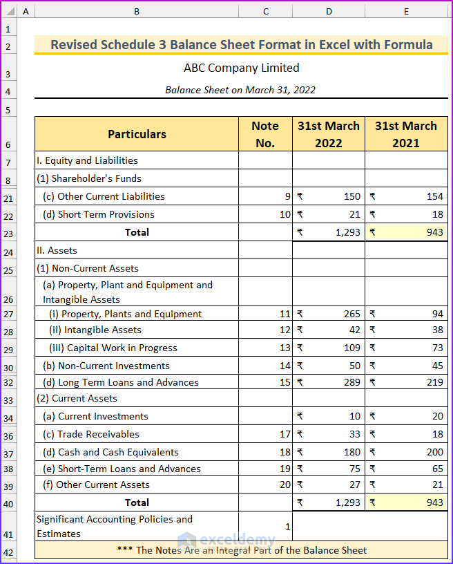
Final Output of Revised Schedule 3 Balance Sheet Format in Excel with Formula

Read More: Schedule 6 Balance Sheet Format in Excel


Basic Balance Sheet Format in Excel

In this section, we will describe the steps to create a basic balance sheet format in Excel with a formula. We will again use the SUM function to calculate the total values.

Steps:

  • Firstly, type the following details to create the balance sheet format.
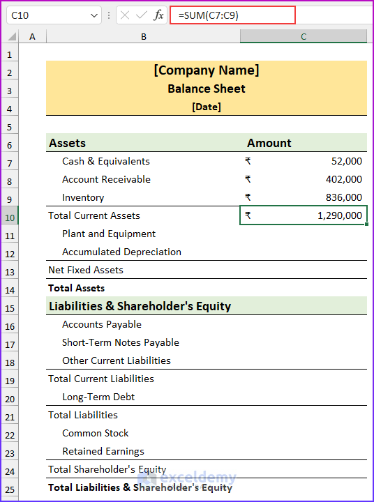
  • Secondly, insert the relevant values and type this formula to find the value of total current assets.

=SUM(C7:C9)

Basic Balance Sheet Format in Excel with Formula

  • Thirdly, type another formula to find the values of the total assets.

=SUM(C10,C13)
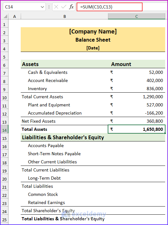
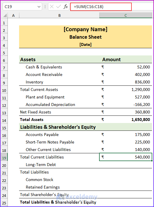
  • Fourthly, type this formula to return the total current liabilities.

=SUM(C16:C18)

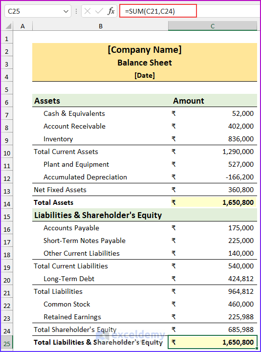
  • Finally, type this formula in cell C25 to calculate the values of total liabilities and shareholder’s equity. Moreover, we can see the balance sheet balances.

=SUM(C21,C24)

Read More: How to Create Vertical Balance Sheet Format in Excel


Things to Remember

  • This balance sheet format in Excel based on the revised Schedule 3 should be used as a practice tool. This should not be the basis for your financial records. You should consult with a chartered accountant after preparing the balance sheet.
  • The values are in crores and arbitrary.

Download Practice Workbook

You can download the Excel file from the link below.


Conclusion

We have shown you three quick steps on how to create a revised Schedule 3 balance sheet format in Excel with the formula. If you face any problems regarding these methods or have any feedback for me, feel free to comment below. However, remember that our website implements comment moderation. Therefore, your comment may not be instantly visible. So, have a little bit of patience, and we will solve your query as soon as possible. Thanks for reading, keep excelling!


<< Go Back to Balance Sheet | Finance Template | Excel Templates

Get FREE Advanced Excel Exercises with Solutions!
Rafiul Haq
Rafiul Haq

Rafiul Haq worked as an Excel and VBA Content Developer in Exceldemy for over two years and published almost 200 articles for the website. He is passionate about exploring new aspects of Excel and VBA. He received his Bachelor of Science in Mechanical and Production Engineering (MPE) from the Islamic University of Technology. Rafiul furthered his education by obtaining an MBA in Finance from the Institute of Business Administration (IBA) at the University of Dhaka. Apart from creating... Read Full Bio

We will be happy to hear your thoughts

Leave a reply

Advanced Excel Exercises with Solutions PDF


ExcelDemy
Logo