How to Create a Balance Sheet Format in Excel with Formulas

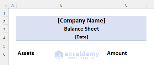
Step 1 – Create a Proper Heading for the Balance Sheet

• In cell B2, type the name of your company.
• In cell B3, write Balance Sheet.
• Enter the date in cell B4.
• Merge cells B and C for rows 2 to 4.
• Apply the Bottom Border from the Home tab.
• Your balance sheet heading will now look as follows.

Step 2 – Insert Balance Sheet Components

• In Column B, enter the components: Assets, Liabilities, and Shareholder’s Equity.
• Corresponding amounts will be entered in Column C.

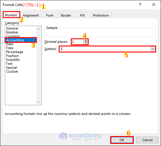
Step 3 – Format the Amount Column

• Before entering data, format the Amount column.
• Select Column C by clicking on the column number.
• Press CTRL+1 to open the Format Cells dialog box.
• Choose the Accounting number format with 2 decimal places.
• Ensure the $ sign is visible.
• Click OK.

Read More: How to Create Tally Debit Note Format in Excel

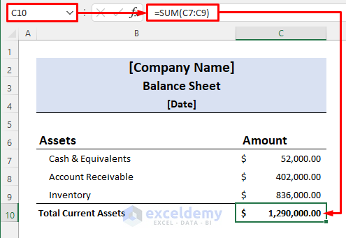
Step 4 – Insert Current Assets

• Enter the current assets into your balance sheet. These are typically assets with a period of less than one year. Examples include Cash and Equivalents, Accounts Receivable, and Inventory.
• In cells B7 to B9, enter the names of these components.
• Corresponding amounts should be entered in cells C7 to C9.
• To calculate the total current assets, enter the formula in cell C10:

Step 5 – Input Fixed Assets

• Enter the fixed assets (such as Plant & Equipment) in cell B11.
• The corresponding amount should be entered in cell C11.
• Depreciation amounts must be entered as negative values (inside brackets).
• Calculate the Net Fixed Assets using the formula in cell C13:

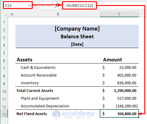
Step 6 – Calculate Total Assets

• In cell C14, calculate the Total Assets by adding the Total Current Assets and Net Fixed Assets:

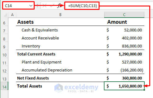
Read More: Revised Schedule 3 Balance Sheet Format in Excel with Formula

Step 7 – Input Current Liabilities

• Enter the current liabilities (such as Accounts Payable, Short-Term Notes Payable, etc.) in cells B16 to B18.
• Corresponding amounts should be entered in cells C16 to C18.
• Calculate the total current liabilities using the formula in cell C19:

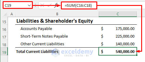
Step 8 – Estimate Total Liabilities

• Enter the long-term liabilities (such as Long-Term Debt) and their corresponding values.
• Calculate the total liabilities using the formula in cell C21:

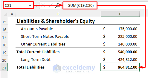
Step 9 – Calculate Total Shareholder’s Equity

• Enter the Shareholder’s Equity components (Common Stock, Treasury Stock, Retained Earnings, etc.), also known as Owner’s Equity.
• In cell C24, calculate the total shareholder’s equity:

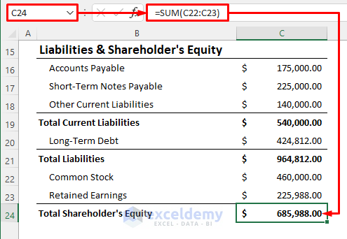
Read More: Schedule 6 Balance Sheet Format in Excel

Step 10 – Estimate Total Liabilities & Shareholder’s Equity

• In cell C25, enter the following formula to find the Total Liabilities & Shareholder’s Equity. Ensure that this value matches the total assets obtained earlier:

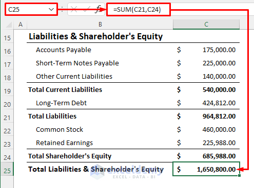
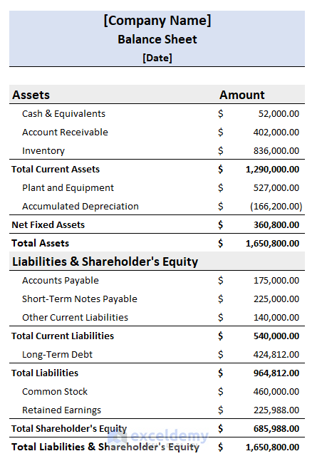
Step 11 – Prepare Final Balance Sheet

• Apply any necessary fill color or other formatting as required.
• After completing these steps, your balance sheet will appear as follows:

Things to Remember

• Always use a negative (-) sign before any depreciation amount.
• Ensure that the total assets, total liabilities, and shareholder’s equity in your balance sheet match.

Download the Free Templates

You can download the practice workbook from here:

Related Articles

• How to Make Hotel Balance Sheet Format in Excel
• Create Horizontal Balance Sheet Format in Excel
• How to Perform Balance Sheet Ratio Analysis in Excel

<< Go Back to Balance Sheet | Finance Template | Excel Templates