In this tutorial, I am going to show you step-by-step procedures to perform balance sheet ratio analysis in Excel. You can quickly use these steps even in large datasets to find different balance sheet ratio values. Throughout this tutorial, you will also learn some important Excel tools and techniques that will be very useful in any Excel-related task.
Step-by-Step Procedures to Perform Balance Sheet Ratio Analysis in Excel
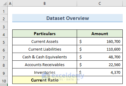
We have taken a concise Excel dataset to explain the steps clearly. The dataset has approximately 6 rows and 2 columns. Initially, we formatted all the cells containing dollar values in Accounting format. For all the datasets, we have 2 unique columns Particulars and Amount. Although we may vary the number of columns later on if that is needed.
Step 1: Finding Current Ratio
This criterion compares the current assets and the current liabilities of a company. This actually indicates whether a firm can cover its short-term debts with its current short-term assets which then shows the firm’s liquidity.
- First, go to cell C10 and insert the following formula:
=C5/C6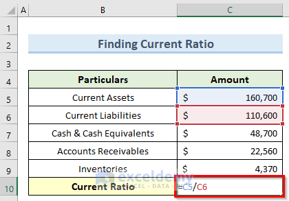
- Now, press Enter and this will calculate the current ratio for the balance sheet.

Read More: How to Create Tally Debit Note Format in Excel
Step 2: Determining Quick Ratio
The Quick Ratio gives an idea of a company’s short-term liquidity condition. It is also known as the Acid Test Ratio. This ratio measures the capability of a company to pay the current liabilities without consuming or selling the inventory. We can calculate the quick ratio by dividing the most liquid assets of a company by total current liabilities.
- To begin with, double-click on cell C10 and enter the below formula:
=(C7+C8)/C6
- Next, press the Enter key and you should get the quick ratio of the balance sheet values.

Read More: Revised Schedule 3 Balance Sheet Format in Excel with Formula
Step 3: Cash Ratio Solving
This ratio gives the indication that a company can cover short-term liabilities using only cash assets. This criterion gives a more conservative result than the ratios before as it only takes into consideration the most liquid assets.
- To begin this method, double-click on cell C10 and insert the formula below:
=C7/C6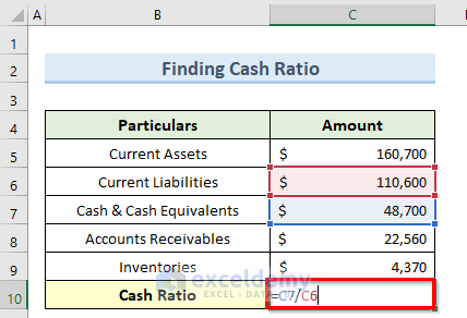
- Next, press the Enter key and consequently, this will find the Cash Ratio inside cell C10.

Read More: Balance Sheet Format in Excel with Formulas
Step 4: Finding Debt to Equity Ratio
We can find this ratio by dividing the total liabilities by the total shareholder’s equity. If the value of this ratio is below 2, then this is generally a good indication for a company. Paying loans, increasing profits, etc. can lower this ratio.
- To start this method, navigate to cell C10 and type in the following formula:
=C6/C9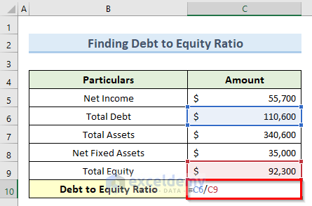
- After that, press the Enter key or click on any blank cell.
- Immediately, this will give you the debt-to-equity ratio for the dataset.

Read More: Schedule 6 Balance Sheet Format in Excel
Step 5: Determining Debt Ratio
The Debt Ratio is also known as the Debt to Asset Ratio. This indicates the percentage of total assets that the creditor owes to the company. The financial leverage of a company largely depends proportionally on the value of this ratio.
- As previously, insert the below formula inside cell C10:
=C6/C7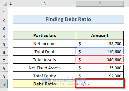
- Finally, press the Enter key and you should get the debt ratio value.

Step 6: Solving for Interest Coverage Ratio
This is the ratio of the EBITDA and the Interest Expense. The EBITDA stands for earnings before interest, taxes, depreciation, and amortization. The higher the value of this ratio, the better it is for the company although this is not a universal criterion. To find this ratio:
- Firstly, navigate to cell C10 and insert the following formula:
=C5/C7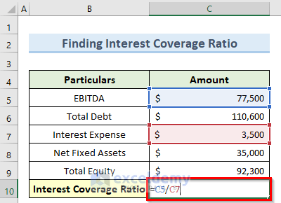
- After that, press the Enter key and immediately this will give the balance sheet Interest Coverage Ratio inside cell C10.

Download Practice Workbook
You can download the practice workbook from here.
Conclusion
I hope that you were able to apply the steps that I showed in this tutorial on how to perform balance sheet ratio analysis in Excel. As you can see, there are quite a few ways to achieve this. So wisely choose the method that suits your situation best. If you get stuck in any of the steps, I recommend going through them a few times to clear up any confusion. If you have any queries, please let me know in the comments.
Related Articles
- How to Create Vertical Balance Sheet Format in Excel
- How to Make Hotel Balance Sheet Format in Excel
- Create Horizontal Balance Sheet Format in Excel
- How to Add Balance Sheet Graph in Excel
<< Go Back to Balance Sheet | Finance Template | Excel Templates
Get FREE Advanced Excel Exercises with Solutions!

Hi!thanks for explaining this..A balance sheet and profit and loss statement accompanying the above would have been great…
Hi SUNITA,
Thank you for your comment and feedback! I appreciate your suggestion regarding including the profit and loss statement alongside the explanation of the balance sheet ratio analysis. It’s a valuable point, and I completely understand how having those additional financial statements would provide a more comprehensive understanding of the topic.
You can go through our article, How to Make Profit and Loss Account and Balance Sheet in Excel to add the profit and loss statement.
Thank you once again for your input!
Regards,
SHAHRIAR ABRAR RAFID
Team ExcelDemy