Hide Rows in Excel (Using Shortcuts, Commands and VBA)

Get FREE Advanced Excel Exercises with Solutions!

In this context, we will explain approaches to hide rows in Excel. While constructing approaches, we will use the Format command, keyboard shortcut, and Group command. Additionally, we intend to discuss the use of the Toggle button and VBA Macro incorporating VBA code.

Often we need to hide unwanted rows to make the necessary rows worthy. Also, the dataset may contain inappropriate information as well as blank cells. Thus hiding rows is not a choice, rather it is compulsory for professionals.

Download Practice Workbook

Hiding Rows in Excel.xlsm

How to Hide Rows in Excel

1. Use Format Menu to Hide Rows

You can use the Format menu to hide within a single moment.

Initially, click on the row number of a row >> Then drag down the cursor or hold the SHIFT key to select contiguous multiple rows.
To hide rows 10-12, Select the rows 10,11,12 >> Then go to the Home tab >> Next expand the Cells command >> Further expand the Format command >> click on the Hide & Unhide option >> Finally select the Hide Rows option.

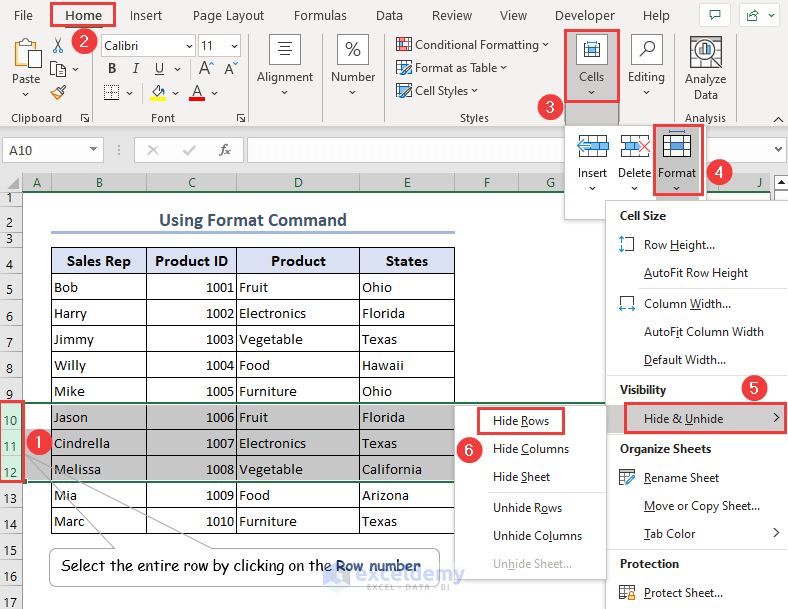
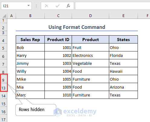
Subsequently, you will be able to hide the 10th, 11th, and 12th rows.

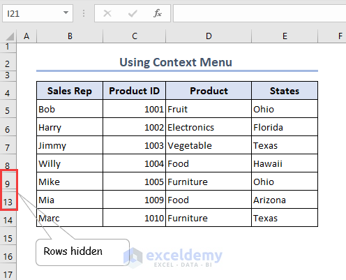
But if you need, you may visit the Format Menu to Unhide Rows article.

2. Hide Rows Using the Context Menu

In this method, we will explore the steps to unhide rows by using the Context menu.

In the beginning, select rows 10 to 12 >> Right-Click on the Mouse to get the Context menu >> Click on the hide option from the Context menu list.

Immediately, we don’t observe the existence of rows 10th, 11th, and 12th.

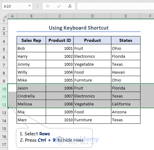
However, you may use the Context Menu to Unhide Rows again if you need.

3. Apply Excel Keyboard Shortcut to Hide Rows

More importantly, you may utilize the keyboard shortcut for hiding rows.

To use the keyboard shortcut you have to select the rows first >> Press CTRL + 9 keys altogether.

Therefore, we get the output hiding rows.

Note: Shortcut for Windows: CTRL + 9 and for Mac: ^ + 9.

Luckily, there is also another shortcut for unhiding rows.

Similar Readings

4. Hide Rows via Excel Group Command

Sometimes we must work with a group of rows and hide grouped rows. Fortunately, you can do this by using the Group command and clicking on the minus sign only.

Primarily, select rows (10-12) >> Then go to the Data tab >> Next expand the Outline command >> Finally, click on the Group command.

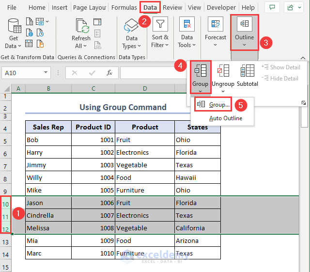
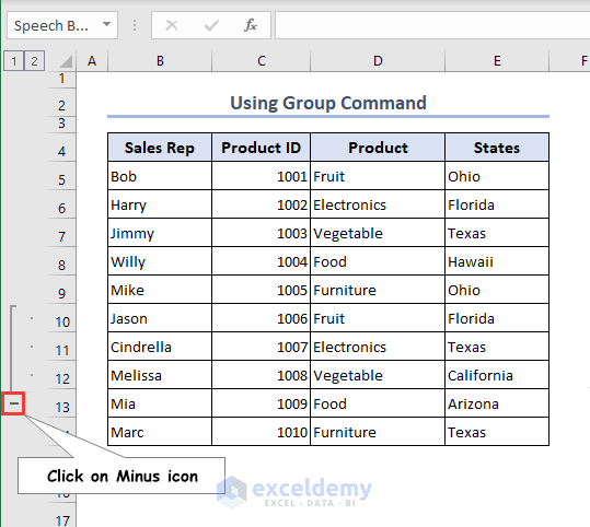
Meanwhile, a Minus (-) sign will be available at the end of the 12th row >> Next, click on the Minus sign.

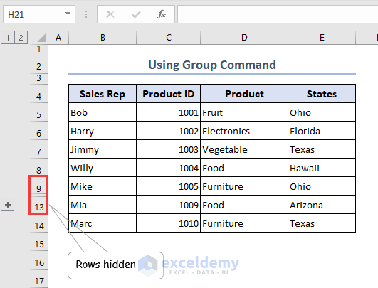
Shortly, you’ll get the following output where the selected rows 10-12 are hidden.

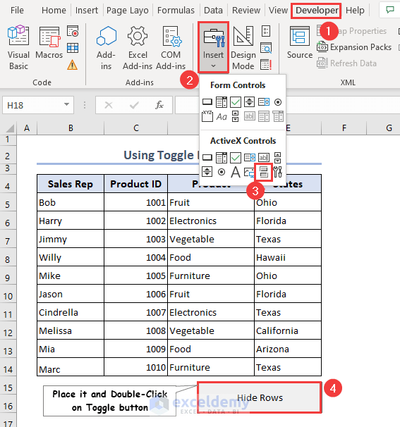
5. Create Toggle Button to Hide Rows

At this time, you’re going to witness an amazing tool by creating a button to hide rows. Thus by clicking on the button, it will automatically hide your selected rows.

Initially, go to Developer tab >> Then Insert button >> Next pick the Toggle Button from the ActiveX Controls section.
Further, locate the Toggle button and re-configure with the VBA code by double-clicking the button.

Enter the following VBA code in the worksheet and hit on the Run icon.

Private Sub ToggleButton1_Click()
Dim xRow As String
xRow = "10:12"
If ToggleButton1.Value Then
    Application.ActiveSheet.Rows(xRow).Hidden = True
    ToggleButton1.Caption = "Unhide Row"
Else
    Application.ActiveSheet.Rows(xRow).Hidden = False
    ToggleButton1.Caption = "Hiding the Selected Rows"
End If
End Sub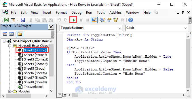

Code Breakdown

In the above code, I declare xRow as a String type.
Then I set the value of xRow as “10:12” as I want to hide rows 10-12.
Eventually, I use the ToogleButton.Value property to specify the object.
Later, Application.ActiveSheet property is used to extract the value of the running sheet.
Right then, Rows(xRow).Hidden is set to True to hide the selected rows, and the same condition (except the Hidden is set to False) was applied to the rest to unhide the rows.

Finally, rows 10-12 are no more visible once we click on the Hide Rows button.

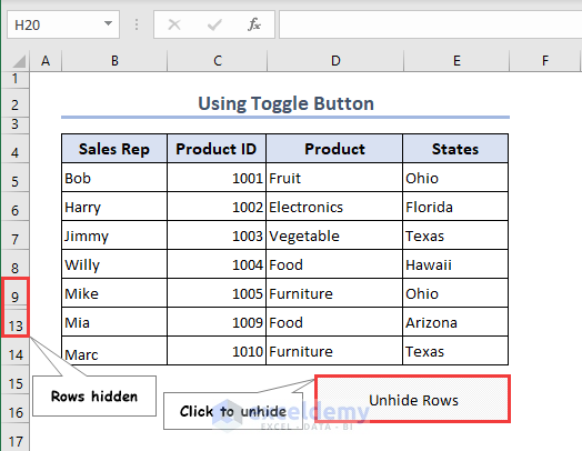
Happily, you’ll get the hidden rows again by clicking on the Unhide Rows button.

6. Hide Rows Applying Excel VBA

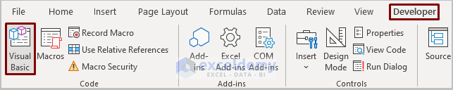
Last but not least, if you want to apply the VBA code to hide rows, you can do that effectively as the code is quite simple. To apply the VBA code, you need to insert a module.

Firstly, open a module by clicking Developer > Visual Basic.

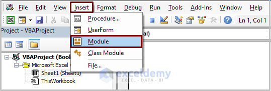
⇰ Secondly, go to Insert > Module.

Now, we will show you three applications with VBA Macro.

6.1. Hide a Single Row

Perhaps, you need to hide a single row e.g. row 10 as shown in the following picture. insert the following code in the VBA module and press the F5 button or hit the Run icon.

Sub Hide_Singe_Row_VBA()
Rows("10").Hidden = True
End Sub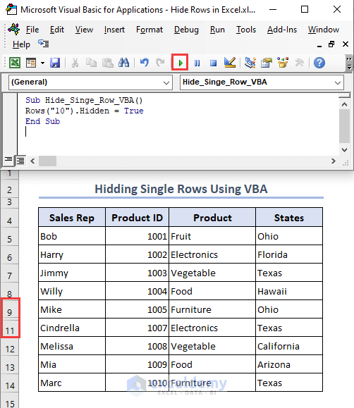

6.2. Hiding Multiple Adjacent Rows Applying VBA Code

In case we require to hide multiple contiguous rows e.g. rows 10-12. By inserting the following VBA code into the created module and clicking on the Run icon or pressing the F5 button, we obtain the obtain as you can see in the image.

Sub Hide_Adjacent_Rows_VBA()
Rows("10:12").Hidden = True
End Sub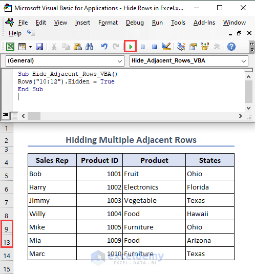

6.3. Hiding Multiple Non-Adjacent Rows Applying VBA Code

If you want to hide multiple rows but they are not contiguous e.g. rows 5-6 & rows 9-11, you can use this method by inserting the following code in the VBA module and press the F5 button or hit the Run icon.

Sub Hide_NonAdjacent_Rows_VBA()
Rows("5:6").Hidden = True
Rows("9:12").Hidden = True
End Sub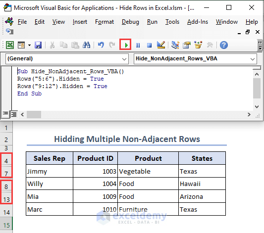

Also, you may use the VBA code to unhide rows.

How to Hide Rows Containing Blank Cells in Excel

1. Apply Filter Feature

Users can quickly filter out and hide the blank cells using the Filter tool.

To filter the B4:E14 range, select the B4:E4 range >> Go to the Data menu >> Expand the Sort & Filter command >> click on the Filter command.

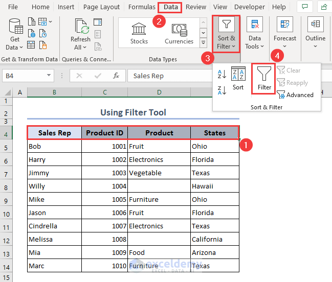
Next, expand the drop-down box >> De-select the Blanks option from the list.

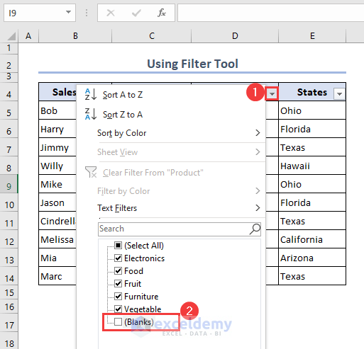
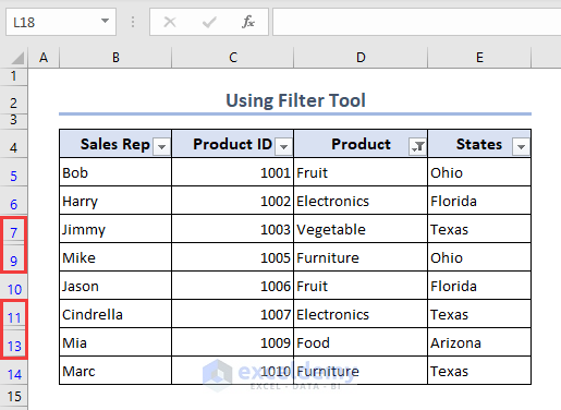
Therefore, rows 8th and 12th containing blanks are hidden.

2. Use Find and Replace Tool

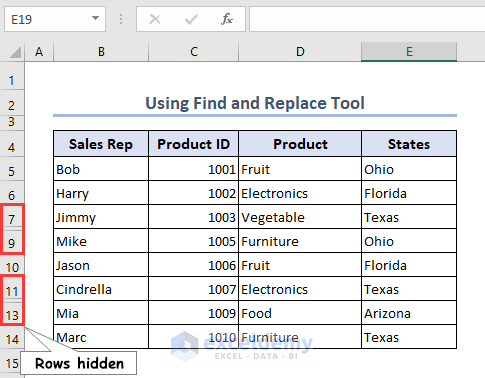
You can figure out the positions of blank cells using the Find and Replace tool.

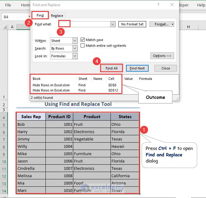
Select the B4:E14 range >> Press Ctrl + F to open the Find and Replace dialog.
From the Find and Replace dialog, go to the Find tab >> Leave blank the Find what field >> Click on the Find All button.
Thus 2 cells having blanks appears.

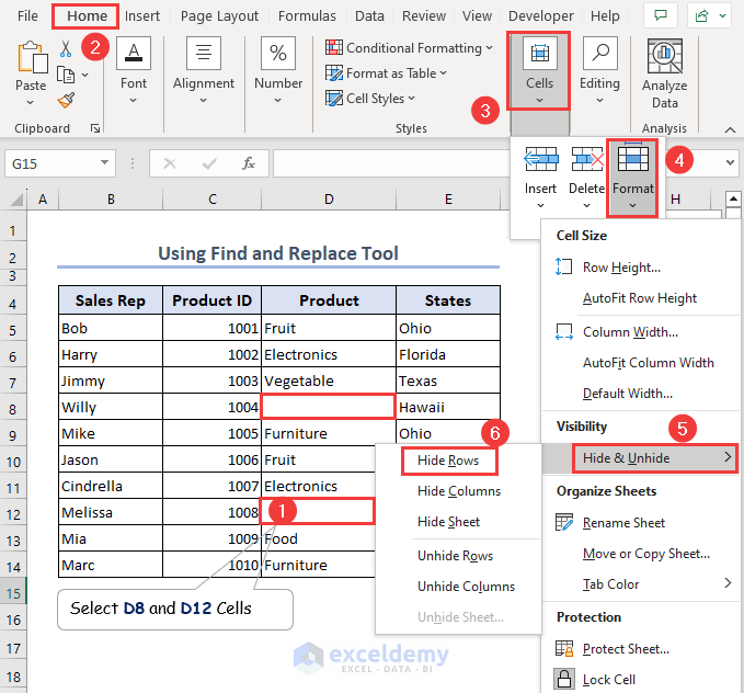
Further, select the blanks D8 and D12 >> Go to the Home tab >> Expand the Cells command >> Expand the Format command >> Click on the Hide & Unhide option >> Select the Hide Rows option.

Therefore, we obtain the result hiding the rows containing blank cells.

3. Apply Go To Special Tool

With the help of the Go to Special tool, you can navigate the blank cells. Thus it will be easier for us to hide those rows.

To begin the process, select the B4:E14 range >> Press the Ctrl + G to open the Go To dialog >> Click on the Special button.

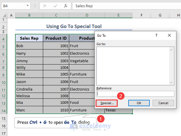
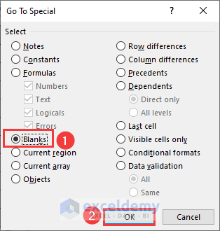
Thus Go To Special dialog appears. Choose Blanks >> Select the OK button.

Next, select the blanks D8 and D12 >> Go to the Home tab >> Expand the Cells command >> Expand the Format command >> Click on the Hide & Unhide option >> Select the Hide Rows option.

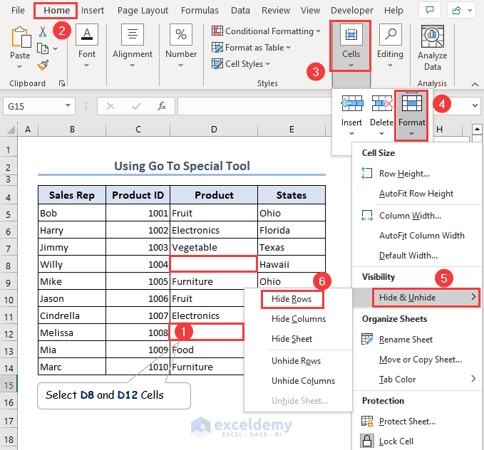
In the end, we obtain the outcome by hiding the blank cells.

How to Unhide Rows in Excel

1. Use Format Command

Like hiding rows, you can also unhide rows by using the Format command of the Home tab.

Initially, Select the B4:D14 range >> Go to the Home tab >> Expand the Cells command >> Expand the Format command >> Click on the Hide & Unhide option >> Select the Unhide Rows option.

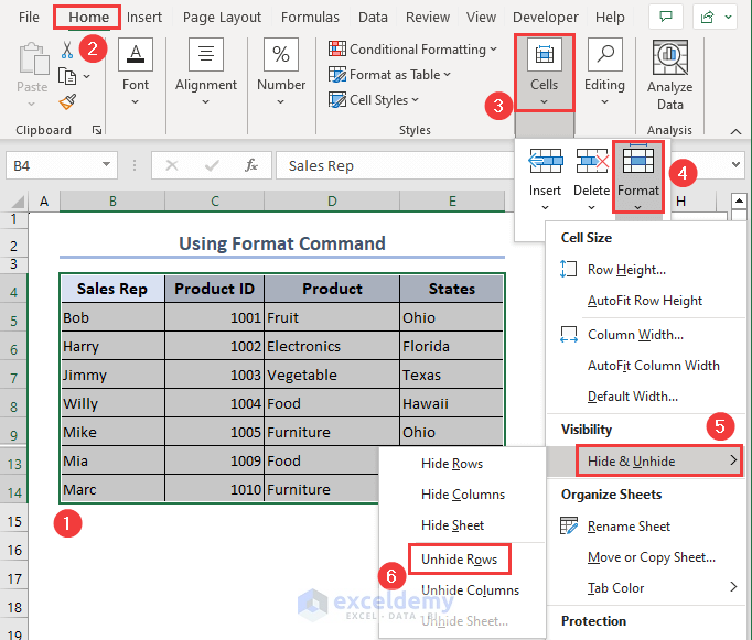
Thus we obtain unhidden rows.

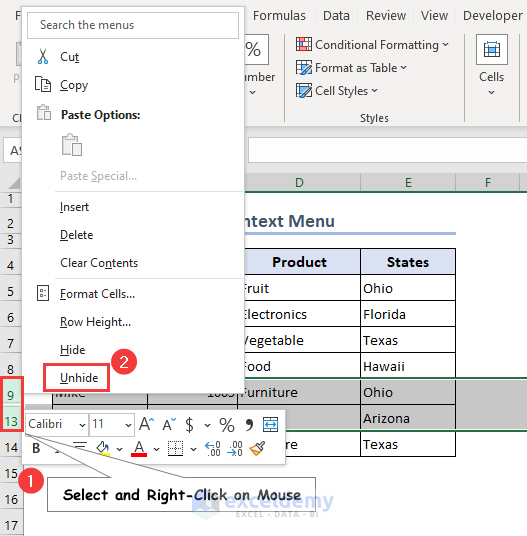
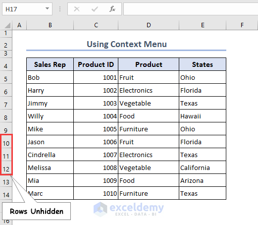
2. Use Context Menu

Users can unhide rows by using the Context menu.

In the beginning, select rows 9 to 13 >> Right-Click on the Mouse to get the Context menu >> Click on Unhide option from the Context menu list.

As you can see in the image we obtain unhidden rows.

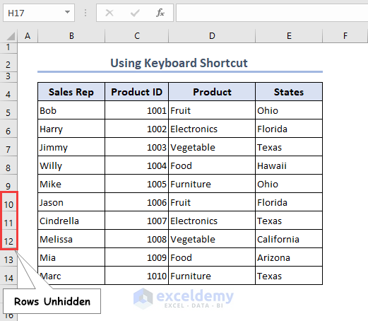
3. Apply Keyboard Shortcut

Application of the keyboard shortcut can accelerate you to unhide the hidden rows.

Initially, select rows 9 to 13 >> Press the Ctrl + Shift + 9 keys to unhide the rows.

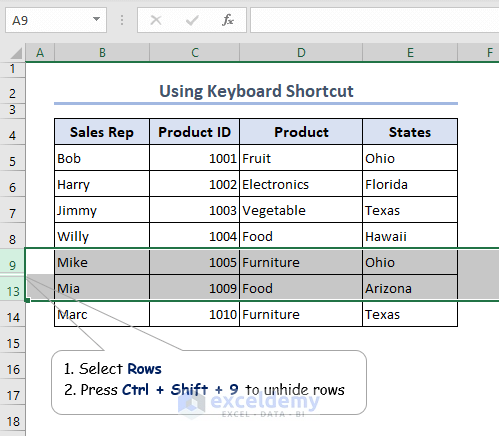
Therefore, we achieve the unhidden rows as you can observe in the image.

Frequently Asked Questions (FAQs)

Q1. How do I hide specific rows in Excel?

Using the Find and Replace dialog you can find the specific data from the data range and hide the rows. From the Find and Replace dialog, go to the Find tab >> Insert text/numbers in the Find what field >> Click on the Find All button. Thus specific cells will be shown >> Then, press Ctrl + 9 to hide rows.

Q2. What is the shortcut to hide rows or columns in Excel?

Press Shift + 9 to hide rows whereas Shift + 0 for columns.

Q3. How to hide rows based on condition in Excel?

Users can hide rows based on conditions automatically by using the Excel VBA code with a suitable condition. However, using Filter or Find tool, one can figure out cells based on condition and hide rows manually.

Q4. Can Conditional Formatting hide rows in Excel?

No, the Conditional Formatting can’t hide or change height rows. Rather it allows specific conditions to highlight cells. To hide rows based on condition, you require to use a VBA code.

Hide Rows in Excel: Knowledge Hub

Conclusion

In short, you may hide rows in Excel utilizing the above methods. Further, if you are keen enough to learn some advanced approaches to hide unhide rows, you can follow the resources from the Knowledge Hub section. Please use the comment section below to leave your thoughts. However, any suggestions regarding the article are appreciated.