[Fixed!] Excel Rows Not Showing but Not Hidden (3 Reasons & Solutions)

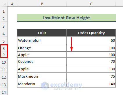
Reason 1 – Unhidden Rows Are Not Visible Due to Insufficient Row Height in Excel

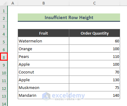
Let’s assume we have a dataset containing several fruits and their order quantities. In this dataset, we cannot see rows 7 and 8. If you look carefully, you will notice a thick line is present between rows 6 and 9. This thick line means rows between rows 6 to 9 have a small height (or even 0). If you try to display rows 7 and 8 using the traditional Unhide option, it won’t work.

Solution:

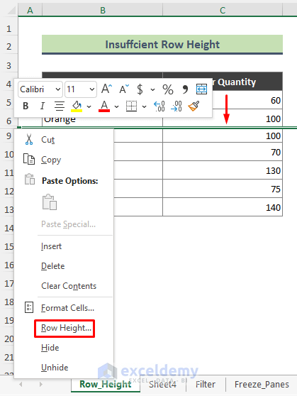
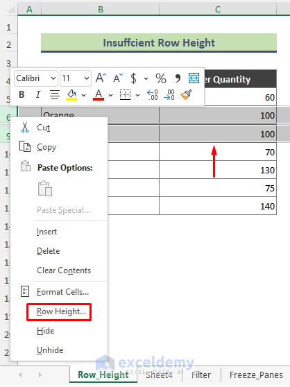
• Put the cursor between rows 6 and 9 and right-click on it.
• Click on the Row Height option.

• The row height dialog appears where you can see that row height is zero (0).

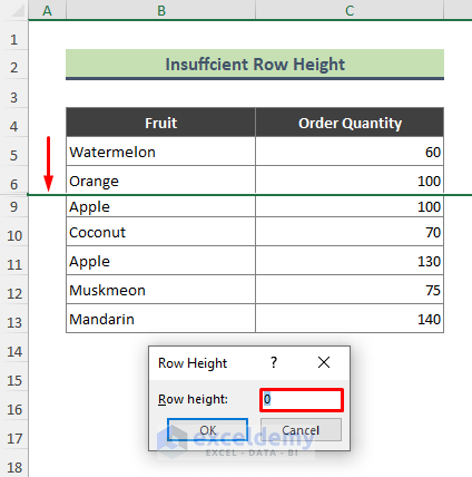
• To make the rows visible, enter the desired height (such as 20) in the Row Height field and press OK.

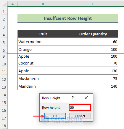
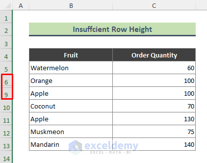
• You will see that row 8 is visible now. Follow the same procedure to display row 7.

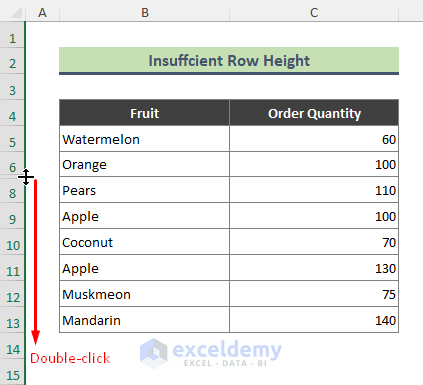
• You can show the shrunk rows by double-clicking on the row header of the regarding row.

• You might not see the thicker line where rows have zero height. In that case, it is better to select corresponding rows and check their height.

• If you want to display rows 7 and 8 at once, select rows 6 to 9 at first. Change their height accordingly.

Read More: VBA to Hide Rows Based on Cell Value in Excel

Reason 2 – Rows Are Not Hidden but Not Displaying When Excel Filter Is Applied

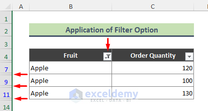
Sometimes when we Filter data in Excel, some rows become invisible. Rows that contain unfiltered data are hidden. You can show invisible rows by withdrawing the applied Filter. For instance, in the below dataset rows 5,6,8, and 10 are not showing as we filtered the dataset for Apple.

Solution:

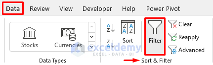
• Go to the corresponding worksheet that contains the data and click any of the cells.

• Go to Data and select Filter.
• Click on the Filter option to disable the filtering.

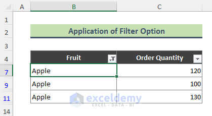
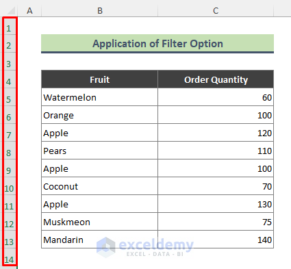
• All the rows in the dataset become visible again.

You can use Ctrl + Shift + L to apply and disable the Filter.

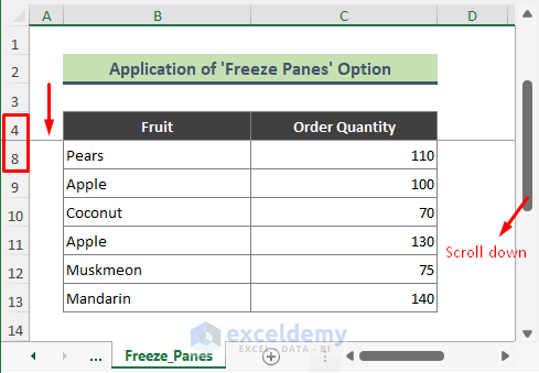
Reason 3 – Excel Rows Are Not Visible Because of Freeze Panes

When we apply the Freeze Panes in Excel and scroll the data, it seems some rows have become hidden. However, these rows are not showing because we scrolled the dataset down after applying Freeze Panes. For example, in the below dataset, we have locked the first four rows by applying Freeze Panes.

Steps:

• Go to the active worksheet and select any cell.
• Go to View, select Freeze Panes, and choose Unfreeze Panes.

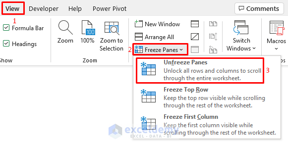
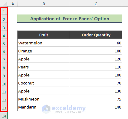
• We can see that all the rows are showing now.

Read More: How to Unhide Top Rows in Excel

Download the Practice Workbook

You can download the practice workbook that we have used to prepare this article.

Related Articles

• [Fix]: Unable to Unhide Rows in Excel
• Unhide All Rows Not Working in Excel
• How to Unhide Rows in Excel
• Shortcut to Unhide Rows in Excel

<< Go Back to Hide Rows | Rows in Excel | Learn Excel