How to Unhide Top Rows in Excel (7 Methods)

To unhide the hidden rows or columns is very common in Excel files. We hide rows or columns intentionally. So, the viewers can not see the information of those cells. In this tutorial, we will discuss how to unhide the top rows in Excel.

The top 3 rows are hidden as we see in the following dataset. We will explain 7 methods to unhide top rows in Excel. Instead of the top 3, we may have any number of top rows hidden. We can solve any of the problems by applying the following methods.

1. Using Format Command in Excel to Unhide Top Rows

We will use the Ribbon shortcut to unhide the top 3 rows of our dataset.

Step 1:

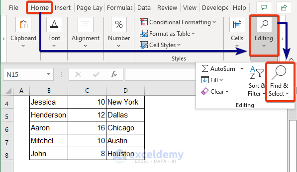
• Go to the Home tab.
• Click Find & Select from the Editing group.

Step 2:

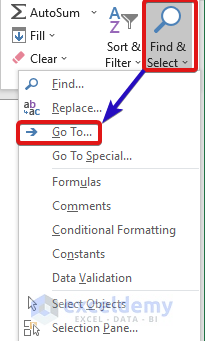
• Select Go To from the options of the Find & Select tool.
• Or we can press Ctrl+G.

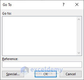
Now, the Go To window will appear.

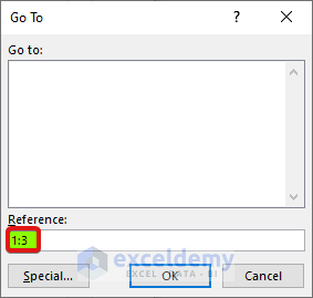
Step 3:

• In the Reference: box put the row references. We put 1:3 according to the hidden rows.
• Then press OK.

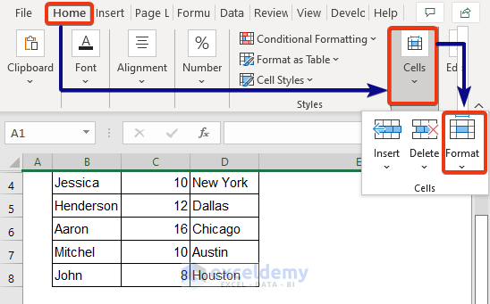
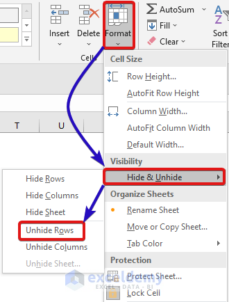
Step 4:

• Now, go to the Cells group from the Home tab.
• Select Format from the option.

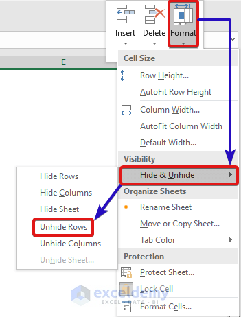
Step 5:

• In the Format tool, go to the Visibility section.
• Choose Unhide Rows from the Hide & Unhide option.

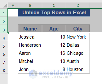
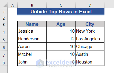
Look at the image below.

Read More: How to Unhide Rows in Excel

2. Clicking with Mouse to Unhide Excel Top Rows

We can easily unhide the top tows using a simple mouse click. This can be performed in two ways. We can unhide all the cells at a time or unhide the rows one by one.

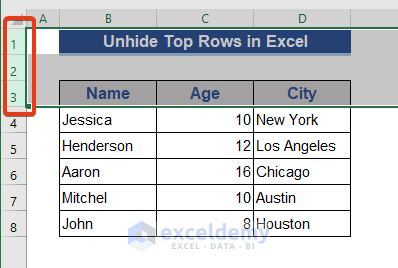
Step 1:

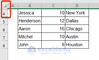
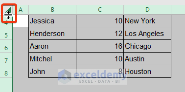
• Our hidden rows are at the top of the dataset. Place the cursor at the top as shown in the following image.

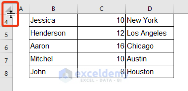
Step 2:

• Double-click the mouse.

Row 3 is showing now.

Step 3:

• Again, place the cursor at the top of the dataset.

Step 4:

• Double-click on the mouse.

Row 2 is showing here.

Step 5:

• Continue this process until any cell is hidden.

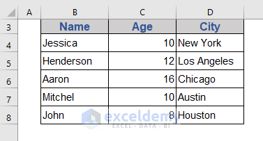
Here, all the top hidden rows are unhidden now.

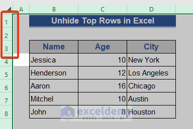
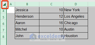
We can also unhide all the top rows at a time. For that, please see the next steps.

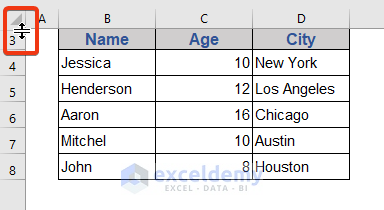
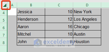
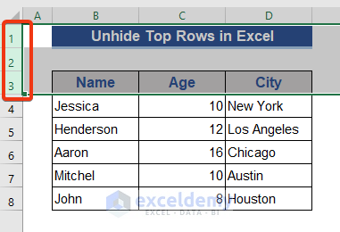
• Click on the triangle box shown in the following image. This selects all the cells.
• Or we can press Ctrl+A to select all the cells.

• Now, place the cursor between the triangle box and the present row.

• Double click the mouse.

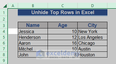
We can see that all the top hidden cells are unhidden now.

One problem we face in this method is that, the row height changes. It may be a problem for somebody.

3. Unhiding Top Rows Using Excel Context Menu

The Context Menu is another way to unhide top rows in Excel.

Step 1:

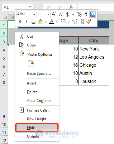
• We need to select all the cells first. Place the cursor on the triangle box marked on the image.
• Or we can press Ctrl+A.

Step 2:

• Press the right button of the mouse.
• Select Unhide option from the context menu.

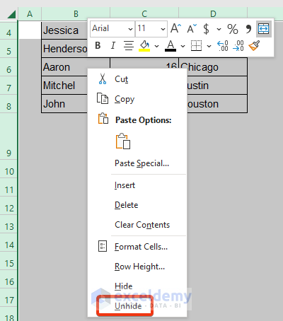
Now, look at the dataset.

All the hidden rows are unhidden now. One noticeable matter is that, the row width of the hidden rows changes. Using this method, not only the top rows but also all hidden rows will unhide.

4. Using Excel Name Box to Unhide Top Rows

Name Box is an excellent option to unhide top rows in Excel.

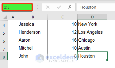
Step 1:

• Click on the Name box.

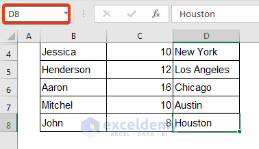
Step 2:

• Hidden rows need to be input here. We put 1:3 in the name box.
• Then press Enter button.

Step 3:

• Click on the Format tool from the Cells group.
• Look at the Visibility segment of Format.
• Choose Unhide Rows from the Hide & Unhide option.

See the following image.

The hidden top rows are presented now.

5. Inserting Keyboard Shortcut to Unhide Top Rows

The keyboard shortcut is the fastest way to unhide the top rows. We can implement this in only two steps.

Step 1:

• Select the whole worksheet by clicking on the triangular box at the top of the sheet.
• Or press Ctrl+A.

Step 2:

• Now, press Ctrl+Shift+9.

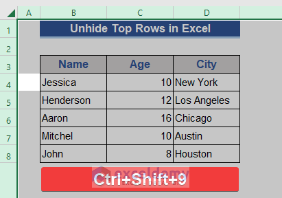
All the top hidden rows are visible now. This method can visible all the hidden rows.

Read More: Shortcut to Unhide Rows in Excel

6. Changing Row Height to Uncover Top Rows

This is another fast method to uncover the hidden top rows.

Step 1:

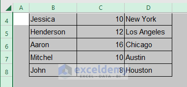
• Select the whole dataset by pressing Ctrl+A.

Step 2:

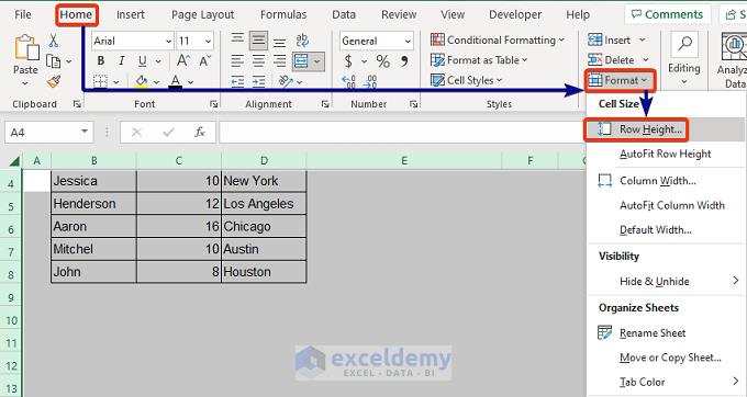
• Go to the Format tool from the Home tab.
• Click on Row Height from the Format option.

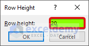
Step 3:

• Row Height window will appear. Put 20 as height.
• Then press OK.

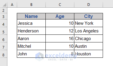
Now, look at the following image.

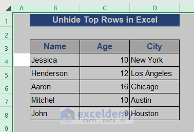
The top hidden rows are visible now. Also, need to add that all hidden rows will be visible with this method. The row height will be uniform for that worksheet.

7. Applying Excel VBA to Disclose Top Rows

Here, we will apply an Excel VBA code to disclose the top rows shortly.

Step 1:

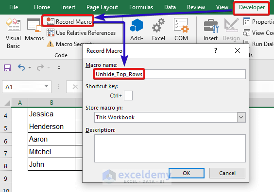
• Go to the Developer tab first.
• Choose Record Macro from the Code group.
• Put a name on the Macro name box.
• Then press OK.

Step 2:

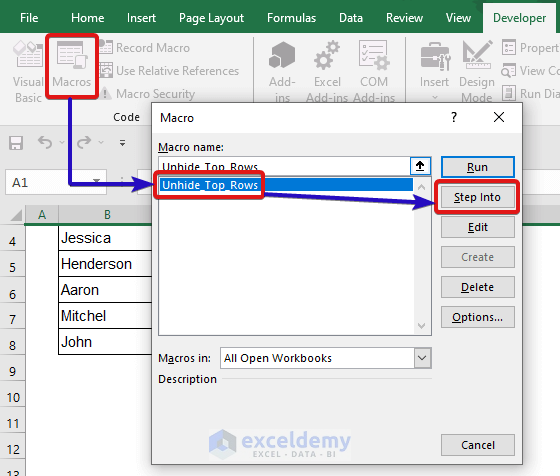
• Now, click on Macros.
• Select the marked Macro from the list and then Step Into it.

Step 3:

• Put the following VBA code on the command module.

Sub Unhide_Top_Rows()
ActiveSheet.Range("1:3").EntireRow.Hidden = False
End Sub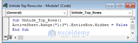

Step 4:

• Now, click on the marked box to run the code or press F5.

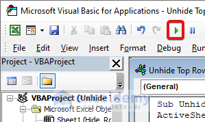
Now, look at the following image.

The top unhidden rows are visible now.

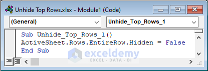
If we have hidden rows only in top cells, through the whole dataset, we may run the below code.

Sub Unhide_Top_Rows_1()
ActiveSheet.Rows.EntireRow.Hidden = False
End Sub

Read More: Excel VBA: Unhide All Rows in Excel

How to Hide Top Rows in Excel?

We’ve learned so far how to unhide top rows in Excel with 7 easy methods. Now if you’re unsure of the procedure to hide the rows then we’ll cover this topic in this section too. We will hide the top 3 rows from here.

Step 1:

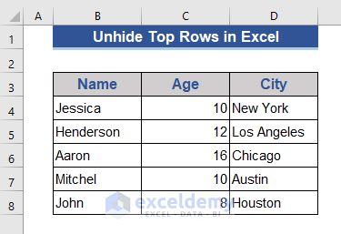
• Select top 3 Row 1,2,3 are our top rows here. Select by pressing the Ctrl (select one by one) or Shift (select first and last rows) keys.

Step 2:

• Click the right button on the mouse.
• Select Hide from the dropdown list.

Notice the following image.

Here, we can see that the top 3 are hidden.

Things to Remember

• Ctrl+Shift+0 shortcut applicable for unhide column from the dataset.
• In the Name box method, we may use cell references instead of rows.
• Some methods will change the row height.

Download Practice Workbook

Download this practice workbook to exercise while you are reading this article.

Conclusion

In this article, we described 7 methods to unhide top rows in Excel. Some methods may be applied to unhide rows from the whole dataset. I hope this will satisfy your needs. Please, give your suggestions in the comment box.

Related Articles

• [Fix]: Unable to Unhide Rows in Excel
• Unhide All Rows Not Working in Excel
• [Fixed!] Excel Rows Not Showing but Not Hidden

<< Go Back to Hide Rows | Rows in Excel | Learn Excel