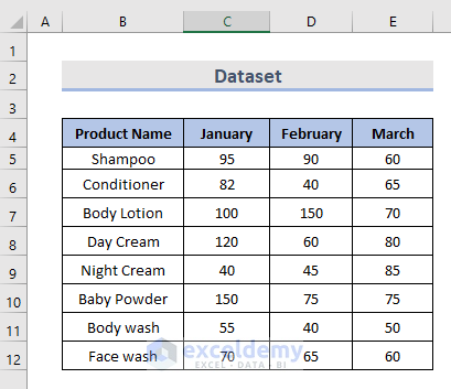
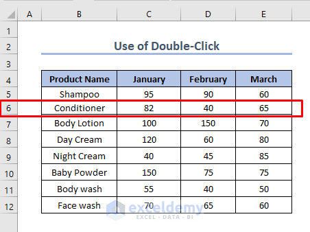
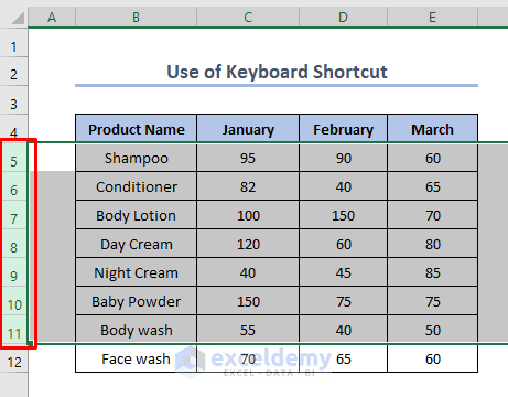
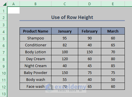
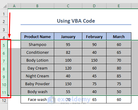
The sample dataset showcases item names and sales from January to March.
Method 1 – Show Hidden Rows Using the Context Menu in Excel
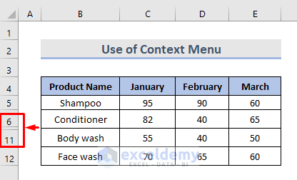
Steps:
Select the rows: one above and one row below the row or rows you want to see. Right-click and choose unhide..

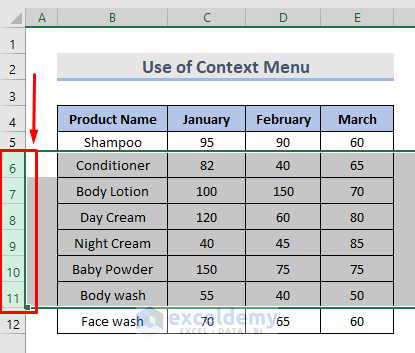
This is the output.
Method 2 – Unhide Rows by Double Clicking
Steps:
- Place the cursor over the hidden row and double-click until a split two-headed arrow is displayed.
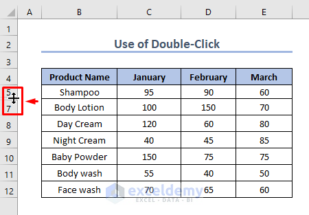
The row is visible.
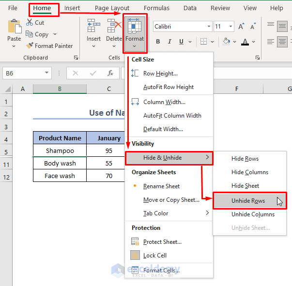
Method 3 – Unhide Rows using the Format Feature
Steps:
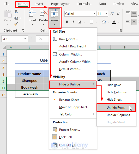
- Select the rows you want to unhide.
- Go to the Home tab > Cells > Format > Hide & Unhide.
- Click Unhide Rows.
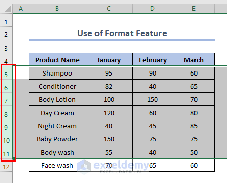
Hidden rows are visible.
Read More: [Fixed!] Excel Rows Not Showing but Not Hidden
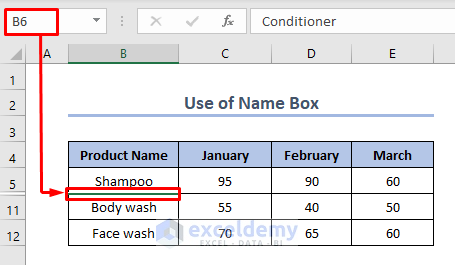
Method 4 – Unhide a Specific Row Using the Name Box in Excel
Steps:
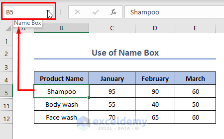
- Enter B6 in the name box.
- Press Enter.
- The green line indicates B6 is selected.
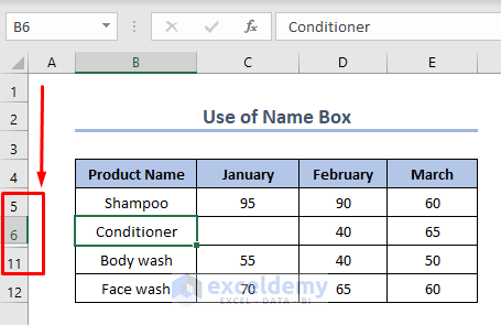
- Go to the Home tab > Format > Hide and Unhide > Unhide Rows.
The whole row containing B6 is visible.
Method 5 – Disclose Rows using a Keyboard Shortcut
Steps:
- Select the hidden rows including one row above and one below.
- Press Ctrl, Shift, 9.
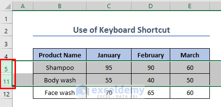
Hidden rows will be displayed.
Read More: Shortcut to Unhide Rows in Excel
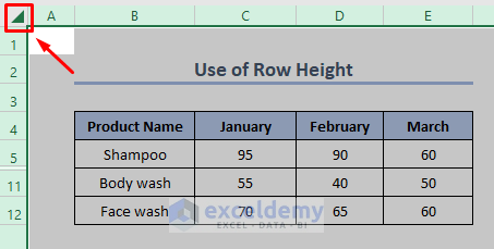
Method 6 – Making Rows Visible by Changing the Row Height
Steps:
- Click the top left corner and select the whole spreadsheet.
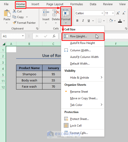
- Go to the Home tab and choose Format .
- Select Row Height.
- In the new window, enter a row height. Here, 18.
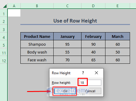
Hidden rows will be displayed.
Method 7 – Show All Hidden Rows in the Whole Excel Spreadsheet
Steps:
- Click the top left corner of your sheet.

- Right-click and select Unhide.
Read More: Unhide All Rows Not Working in Excel
Method 8 – Unhide Rows Using a VBA Code in Excel
Steps:
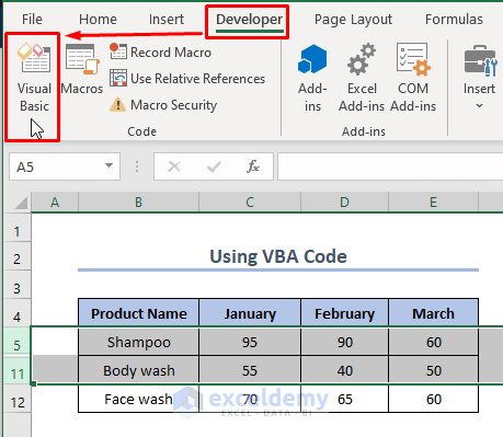
- Select the rows you want to unhide.
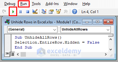
- Go to the Developer tab and choose Visual Basic to open the visual basic editor.
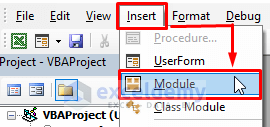
- Click Insert and select ‘Module’. A new module window will open.
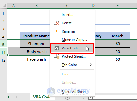
- You can also right-click the spreadsheet bar and go to View Code.
- Enter the VBA code.
VBA Code:
Sub UnhideAllRows()
Selection.EntireRow.Hidden = False
End Sub- Click Run or press F5 to run the macro.
Hidden rows will be displayed.
Check the Number of Hidden Rows
Steps:
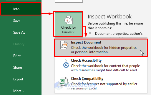
- Select the File tab.
- Go to Info.
- Click ‘Check for Issues‘.
- Click Inspect Document.
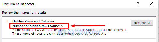
- To make sure the Hidden Rows and Columns option is enabled in the Document Inspector, click Inspect.
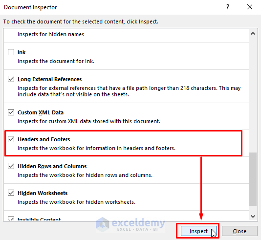
You will see the total number of hidden rows and columns.
Reasons Why Rows in Excel Cannot Be Unhidden
- The Worksheet is protected
Go the Review tab > select Changes > click Unprotect Sheet.
Click Protect Sheet in the Review tab, choose Format rows and click OK to keep the worksheet protected.
- Small Row height, but Not Zero
Check the height of the rows.
- Filtered out Rows
When row numbers become blue, it means that some rows have been filtered. Remove all filters.
Tips:
To unhide all rows and columns, select the entire spreadsheet and press Ctrl + Shift + 9 to see hidden rows. Press Ctrl + Shift + 0 to see hidden columns.
Download Practice Workbook
Download the workbook here.
Related Articles
<< Go Back to Hide Rows | Rows in Excel | Learn Excel
Get FREE Advanced Excel Exercises with Solutions!

Thanks for sharing these methods to unhide rows in Excel! I was particularly impressed with the ‘AutoFit’ method, it wasn’t something I knew existed. Saves me so much time when working with large datasets.
Dear,
You are most welcome.
Regards
ExcelDemy
Could you please add Grouping to this?
I didn’t know what to call it but I’d seen it in spreadsheets and was unsure how to implement it until checking this answer and finding that this wasn’t what I was after. Grouping can hide and display rows and columns and makes it obvious that they can be seen or hidden.
Hello Bill Reid,
You’re absolutely right—Grouping is another great way to manage hidden or displayed rows and columns. It not only lets you collapse/expand sections but also provides a clear visual indicator that rows or columns are grouped. Thanks for pointing this out—we’ll look into adding a section on Grouping to make the article more complete!
Regards
ExcelDemy