Excel Hide Rows Based on Cell Value with Conditional Formatting

In this article, we’re going to show you 2 methods in Excel to hide rows based on cell value conditional formatting. To demonstrate our methods, we’ve picked a dataset with 3 columns: Name, Email, and Born.

How to Hide Rows Based on Cell Value with Conditional Formatting in Excel: 2 Ways

1. Changing Text Color to Hide Rows Based on Cell Value with Conditional Formatting

For the first method, we’re going to set the text color to White to hide rows based on cell value Conditional Formatting. We aim to hide all the rows with the year 1988. To do this –

Steps:

Firstly, select the cell range B5:D10.
Secondly, from the Data tab >>> Conditional Formatting > select “New Rule…”.

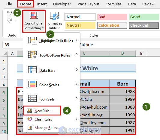
The “New Formatting Rule” dialog box will appear.

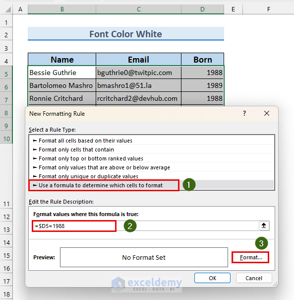
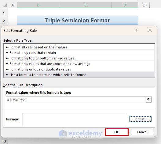
Thirdly, select “Use a formula to determine which cells to format” from the Rule Type section.
Then, type the following formula in the Rule Description section.

=$D5=1988

This will apply our conditional formatting to rows with the year 1988.

After that, select “Format…”

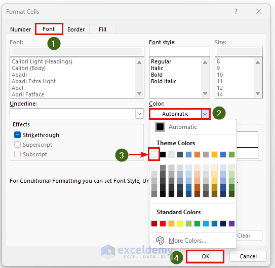
The “Format Cells” dialog box will appear.

Then, from the Font tab >>> Color >>> select “White”.
After that, press OK.

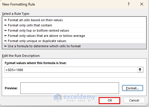
We can see there is nothing inside the Preview box.

Finally, press OK.

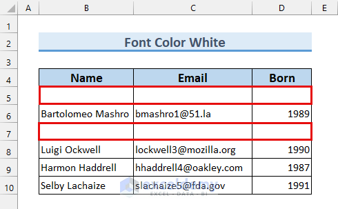
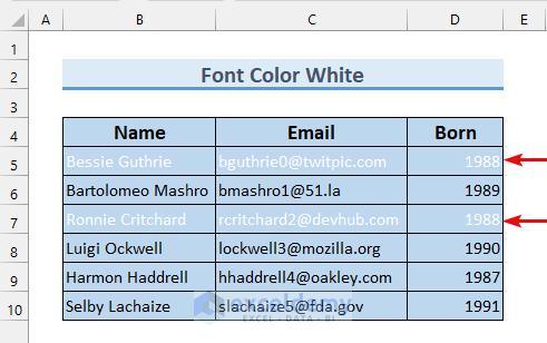
Thus, we’ll hide rows based on cell value conditional formatting. Two rows contained the year 1988, and both of them vanished from view.

Note: This method has a drawback. If we change the background color then the text will appear. Hence, this method is not useful always. However, our next method will solve this problem.

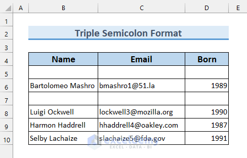
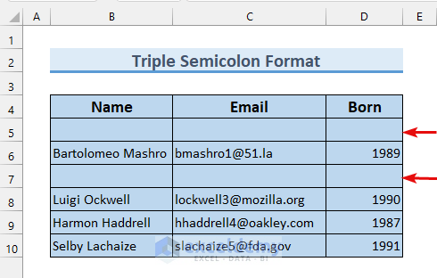
2. Hide Rows Using Conditional Formatting & Custom Format Feature

For this section, we’re gonna use another Conditional Formatting to hide rows based on cell values in Excel. Instead of changing the font color, we’re going to implement a custom formatting, which contains triple Semicolons. Let’s jump into the action.

Steps:

Firstly, following the first method, bring up the “New Formatting Rule” dialog box and click on “Format…”.
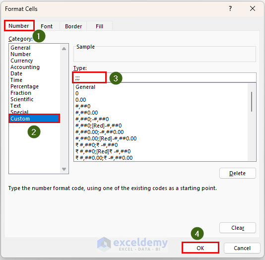
Secondly, from the Number tab >>> select Custom in the Category section.
Thirdly, type triple Semicolons (“;;;”).
Press OK.

We can again notice there is nothing on the Preview box.

Finally, press OK.

In conclusion, this custom format will hide rows based on cell value conditional formatting.

Note: In our previous method, we’ve seen that if we change either the text color from White to any Visible Color or the background color it will make the hidden rows visible. However, using this technique, the rows will not appear, even when we change the background color.

Practice Section

We’ve provided practice datasets for each method in the Excel file. Hence, you can follow along with our methods easily.

Download Practice Workbook

Hide Rows Based on Conditional Formatting.xlsx

Conclusion

We’ve shown you 2 methods in Excel to hide rows based on cell value conditional formatting. If you face any problems, feel free to comment below for further assistance. Thanks for reading, keep excelling!

<< Go Back to Hide Rows | Rows in Excel | Learn Excel

Get FREE Advanced Excel Exercises with Solutions!