How to Hide Rows Based on Cell Value in Excel (5 Methods)

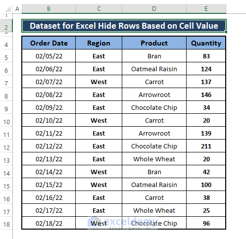
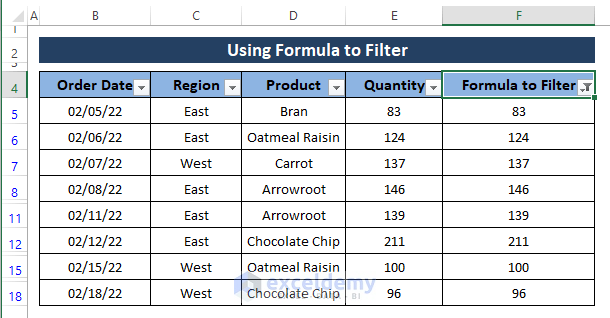
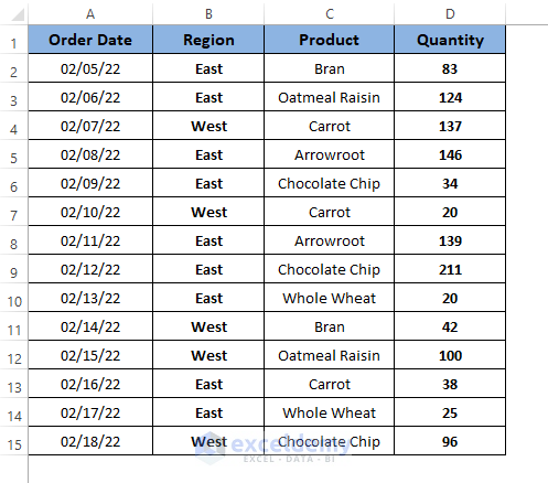
We have a Sales dataset consisting of columns Order Date, Region, Product, and Quantity. We want to use any of the cell values in the column to hide rows.

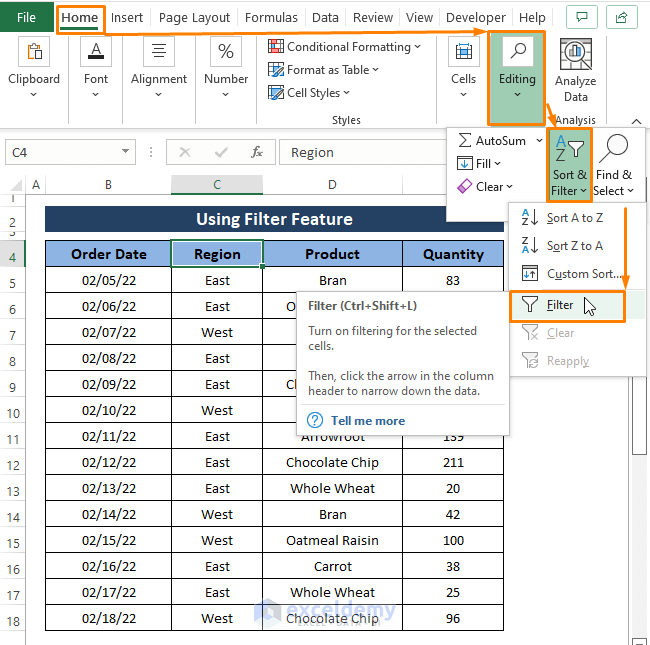
Method 1 – Using the Filter Feature to Hide Rows Based on Cell Value

Steps:

• Go to the Home tab.
• Select Sort & Filter (from the Editing section).
• Select Filter (from the Sort & Filter options).

Selecting Filter displays the Filter icon in each column header.

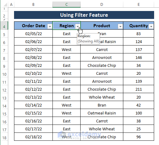
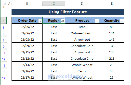
• Click on any filter icon in the column headers (i.e., Region).

• The Filter command box appears. Uncheck any items (i.e., West) to hide their respective rows from the dataset.
• Click on OK.

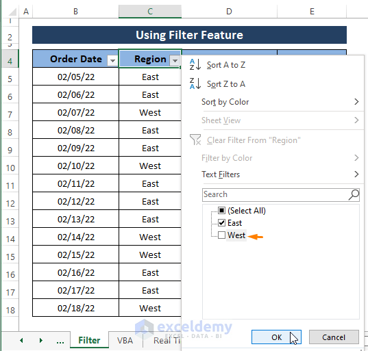
• Excel hides the unticked entries (i.e., West) from the dataset and leaves all other entries on display as shown in the picture below.

Method 2 – Using Formula and Filtering to Hide Rows in Excel Based on Cell Value

We’ll insert a custom string (i.e., Hide) in a helper column based on cell value to indicate whether we need to hide a row.

Steps:

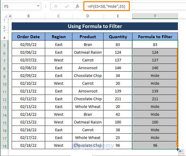
• Use the following formula in the helper cell F5.

The formula returns “Hide” if the respective cell in the E column has a value less than 50, or returns that value otherwise.

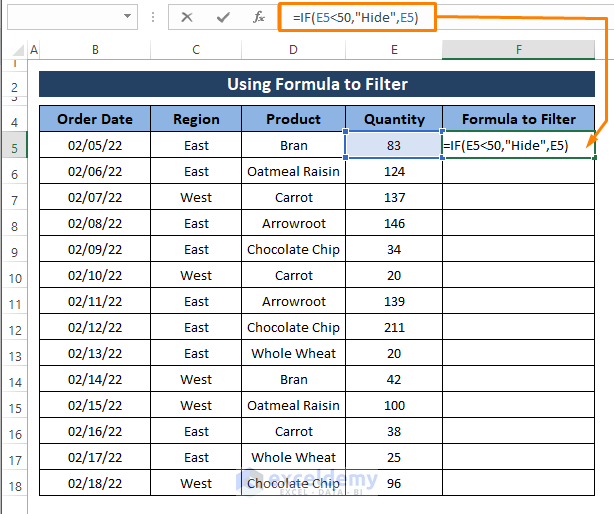
• Press Enter and drag the Fill Handle down to fill all cells in the helper column.

• Follow the Steps of Method 1 to bring out the Filter command box.
• Unselect the Hide value for column F.

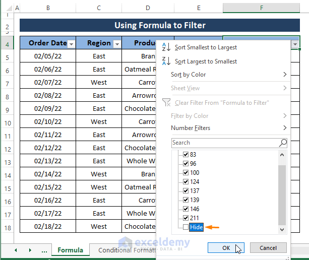
• Here’s the result.

Read More: How to Automatically Hide Rows with Zero Values in Excel

Method 3 – Applying Excel Conditional Formatting to Hide Rows

Steps:

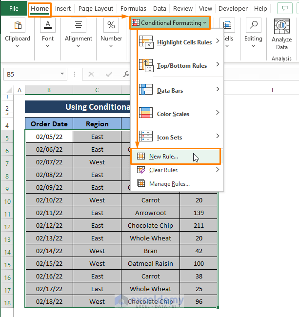
• Go to the Home tab.
• Select Conditional Formatting.
• Select New Rule.

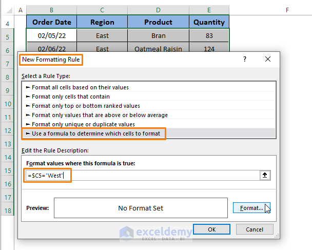
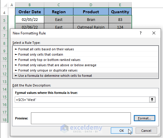
• The New Formatting Rule window appears.
• Select Use a formula to determine which cell to format as Select a Rule Type.
• Insert the following formula under Edit the Rule Description.

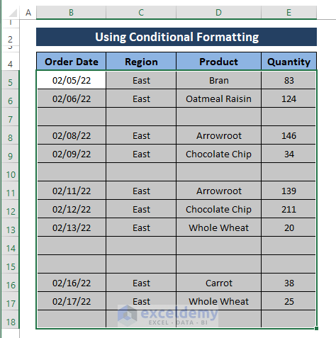
• Click on Format.

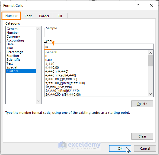
• The Format Cells window appears.
• Select the Number section.
• Choose Custom (under the Category option).
• Type 3 Semicolons (i.e., ;;;) under the Type section.
• Click on OK.

• Excel takes you back to the New Formatting Rule dialog box. Click OK.

• Here’s the result, with all rows that have the value “West” in Region reformatted to not display values.

Method 4 – Hiding Rows Based on Cell Value Using VBA Macro

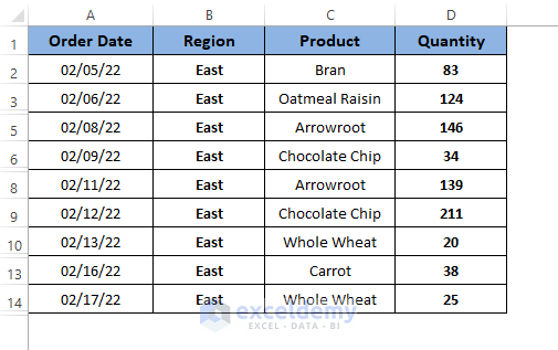
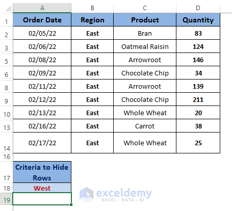
We changed the dataset so it starts from A1 and want to hide the rows depending on a column’s (i.e., Region) value equal to a cell value (i.e., East).

Steps:

• Hit Alt + F11 to open the Microsoft Visual Basic window.
• In the window, select Insert and choose Module.

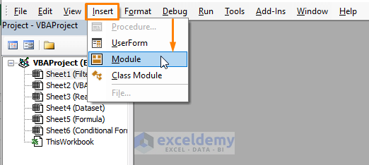
• Paste the following macro code in the Module and press F5 to run the macro.

Sub Hide_Rows_Based_On_Cell_Value()
StartRow = 2
EndRow = 15
ColNum = 2
For i = StartRow To EndRow
If Cells(i, ColNum).Value <> "East" Then
Cells(i, ColNum).EntireRow.Hidden = True
Else
Cells(i, ColNum).EntireRow.Hidden = False
End If
Next i
End Sub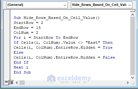

The macro code assigns start (i.e., 2), end (i.e., 15) row and column (i.e., 2, Region Column) numbers. The column number declares in which column the macro matches the given value (i.e., East). Then the VBA IF function hides any rows except the East value existing in the rows of the given column (i.e., Region column).

• Here’s the result.

Read More: VBA to Hide Rows in Excel

Method 5 – Using VBA Macro to Hide Rows Based on Cell Value in Real Time

We created a cell that stores the lookup value that we’ll use to hide rows that contain it.

Steps:

• Open the Microsoft Visual Basic window (by pressing Alt + F11 altogether).
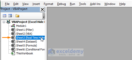
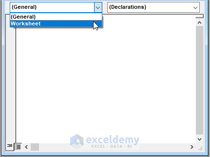
• Double-click on the sheet name (i.e., Sheet3) under the VBAProject section.

• Choose Worksheet from the first drop-down in the code window.

• The Private Sub appears.

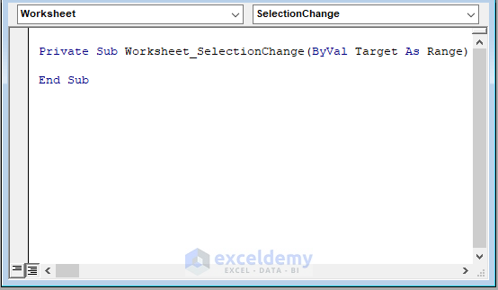
• Paste the following macro code in the code window.

Private Sub Worksheet_SelectionChange(ByVal Target As Range)
StartRow = 2
EndRow = 15
ColNum = 2
For i = StartRow To EndRow
If Cells(i, ColNum).Value = Range("A18").Value Then
Cells(i, ColNum).EntireRow.Hidden = True
Else
Cells(i, ColNum).EntireRow.Hidden = False
End If
Next i
End Sub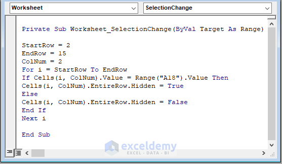

The written macro code assigns start (i.e., 2), end (i.e., 15) row, and column (i.e., 2) numbers. Then it imposes a condition that it hides values equal to cell A18 in column 2. The VBA IF function creates a private macro code to hide rows in real time after entering any value in cell A18.

• Hit F5 to run the macro then go back to the worksheet.
• Type anything that exists in Column B and Press Enter.

• The macro hides the rows that contain that text from the dataset. You can use any text or value of the assigned column to hide rows within a dataset.

Read More: VBA to Hide Rows Based on Cell Value in Excel

Download the Excel Workbook

Related Articles

• How to Hide Blank Rows in Excel VBA
• VBA to Hide Rows Based on Criteria in Excel
• How to Hide the Same Rows Across Multiple Excel Worksheets

<< Go Back to Hide Rows | Rows in Excel | Learn Excel