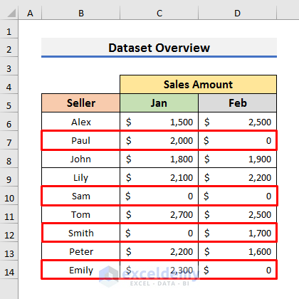
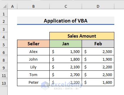
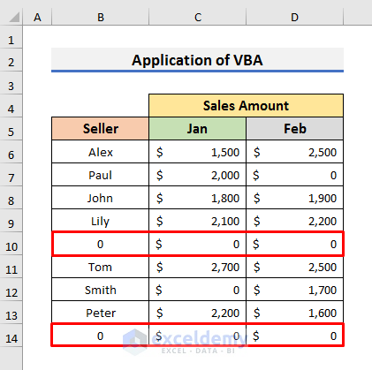
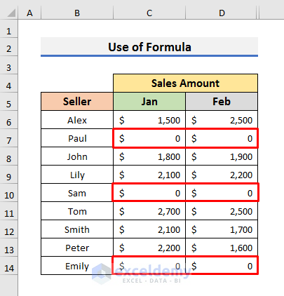
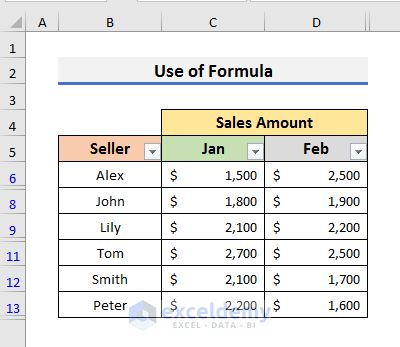
This is the sample dataset.
Method 1 – Apply Excel VBA to Automatically Hide Rows with Zero Values
1.1 With an InputBox
STEPS:
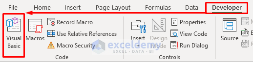
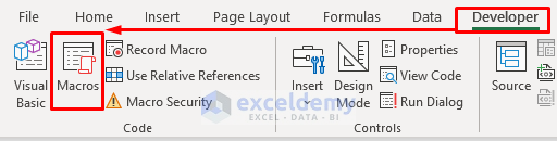
- Go to the Developer tab and select Visual Basic to open the Visual Basic window or press Alt + F11.
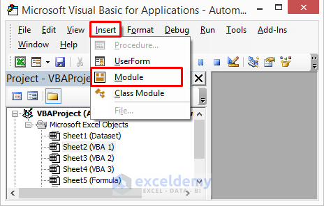
- Select Insert and choose Module.
- In the Module window, enter the code below:
Option Explicit
Sub Hide_Rows_Zero_InputBox()
    Dim cRange As Range
    Dim qq As Range
    Set cRange = Application.InputBox("Specify the Cell Range", _
    "ExcelDemy", Type:=8)
    For Each qq In cRange
        If qq.Value = "0" Then
        qq.EntireRow.Hidden = True
        End If
    Next
End Sub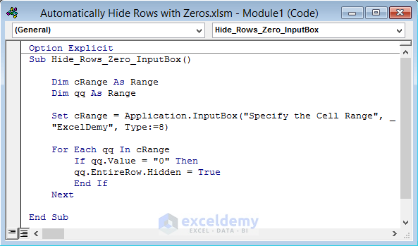
This code hides the entire row if it finds any cell with zero value. Two variables were declared: cRange and qq. The For Next Loop checks whether the cell value equals 0. If it is equal to 0, the entire row is hidden.
- Press Ctrl + S to save the code.
- Press F5 to run the code or go to the Developer tab and select Macros. It will open the Macro window.
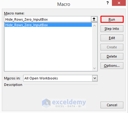
- In the Macro window, select the code and Run it.
- Select the range in which you want to apply the VBA code.
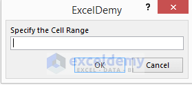
- Click OK.
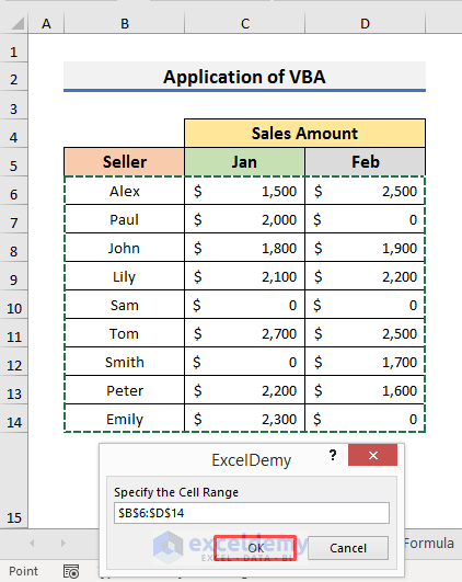
This is the output.
Read More: How to Hide Rows Based on Cell Value in Excel
1.2 Without an InputBox
STEPS:
- Follow the steps in 1.1 to open the Visual Basic window.
- Select Insert >> Module.
- Enter the code below in the Module window:
Option Explicit
Sub Hide_Rows_with_Zeros()
    Dim qq As Range
    For Each qq In Range("B6:D14")
        If Not IsEmpty(qq) Then
            If qq.Value = 0 Then
                qq.EntireRow.Hidden = True
            End If
        End If
    Next
End Sub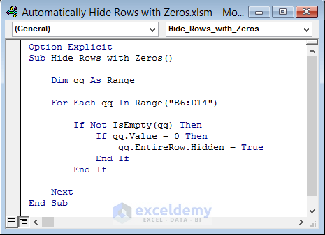
In this code, you need to change the range. Here, B6:D14.
- Press Ctrl + S to save the code.
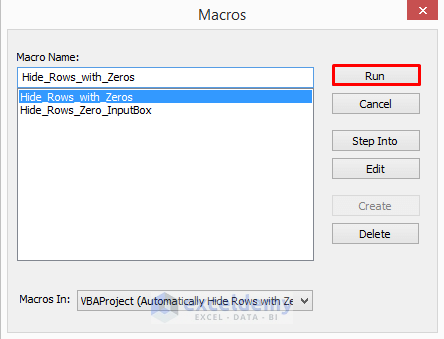
- Press the F5 to run the code.
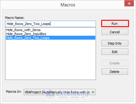
- In the Macros window, select the macro and click on Run.
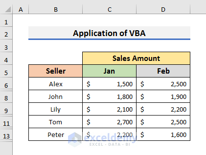
The rows with zero values will be hidden.
Read More: VBA to Hide Rows Based on Cell Value in Excel
1.3 Only When All Values Are Zero
STEPS:
- Follow the steps in 1.1 to open the Visual Basic window.
- Select Insert >> Module.
- Enter the code below in the Module window:
Option Explicit
Sub Hide_Rows_Zero_Two_Loops()
Dim row As Long
Dim col As Long
Dim qq As Boolean
For row = 6 To 14
    qq = True
    For col = 2 To 4
        If Cells(row, col).Value > 0 Then
            qq = False
            Exit For
        End If
    Next col
    Rows(row).Hidden = qq
Next row
End Sub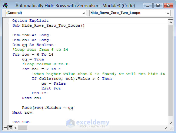
Two For Next Loop were used. The first loop goes row-wise and the second one goes column-wise. They check the cells greater than 0. If all values of a row are 0 then, it hides the entire row.
- Press Ctrl + S to save the code.
- Press the F5 to run the code.
- In the Macros window, select the macro and click on Run.
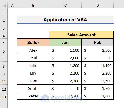
The code will automatically hide rows that contain zero values only in all cells.
Read More: Hide Rows and Columns in Excel
Method 2 – Automatically Hide Rows with Zero Values Using an Excel Formula
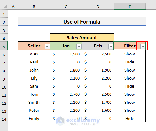
In the dataset below, Rows 7, 10, and 14 contain zero values.
STEPS:
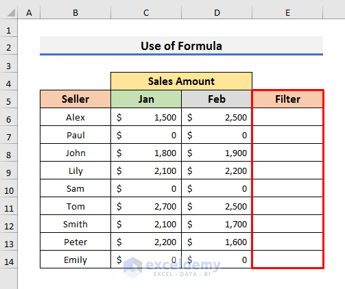
- Add a helper column to insert the formula. Here, Filter.
- Select E6 and enter the formula below:
=IF(COUNTIF(C6:D6,0)=2,"Hide","Show")- Press Enter to see the result.
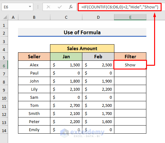
The formula checks if the number of non-zero cells in C6:D6 is 2, using the COUNTIF and theIF functions. If the number of the non-zero cells is greater than 0, the formula will display SHOW in E5. If the number of zero cells is equal to 2, it will display Hide in E5. he IF function.
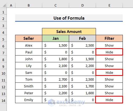
- Drag down the Fill Handle to copy the formula.
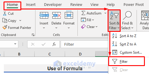
- Go to the Home tab.
- Click Sort & Filter and select Filter.
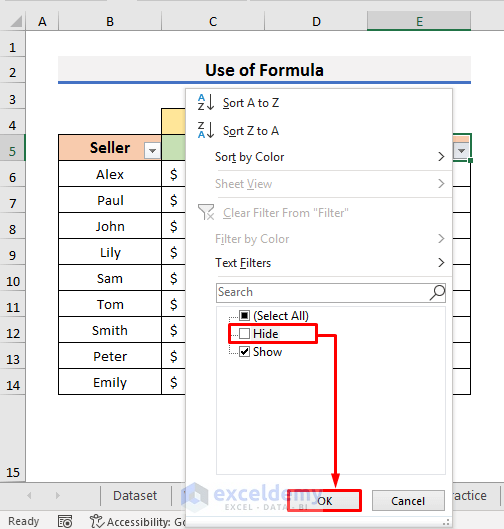
- Click the drop-down arrow in the Filter header.
- Uncheck Hide and click OK.
This is the output.
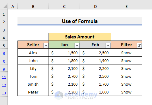
- Hide the helper column.
Read More: Excel Hide Rows Based on Cell Value with Conditional Formatting
Download Practice Workbook
Download the practice book here.
Related Articles
- How to Hide the Same Rows Across Multiple Excel Worksheets
- VBA to Hide Rows Based on Criteria in Excel
- How to Hide Blank Rows in Excel VBA
- VBA to Hide Rows in Excel
<< Go Back to Hide Rows | Rows in Excel | Learn Excel
Get FREE Advanced Excel Exercises with Solutions!

This hides rows that has negative numbers how do I hide rows that are truly zero? Meaning only rows that do not have a negative or positive number.
Hello Frank,
This article contains different methods for different situations. Method 1.3 hides the numbers that are less than Zero. But, if you want to hide zeros only then you can try the following code.
Option ExplicitSub Hide_Rows_With_Zero()Dim row As LongDim col As LongDim qq As BooleanFor row = 6 To 14qq = TrueFor col = 2 To 4If Cells(row, col).Value <> 0 Thenqq = FalseExit ForEnd IfNext colRows(row).Hidden = qqNext rowEnd SubI hope this will help you to solve your problem. Please let us know if you have other queries.
Thanks!