How to Make Balance Sheet in Excel (2 Useful Examples)

Preparing a balance sheet is a must when evaluating an organization. This is because it provides a window into an organization’s financial strengths and weaknesses. With this intention, this article hopes to guide you on how to make a balance sheet in Excel.

Download Practice Workbook

You can download the practice workbook from the link below.

What Is a Balance Sheet? 

In a nutshell, a balance sheet shows the assets and liabilities owned by an organization. In fact, you can tell if a company is making a profit or sinking into debt using the balance sheet.

A balance sheet has two parts, to clarify, the asset part and the liabilities and equities part. Consequently, the two parts can be combined to give the following equation.

Asset = Liability + Equity

Assets consist of resources that generate benefits in the future like equipment, land, buildings, etc.

Liabilities are things that the company owes to a person or a company like cash, loans, etc.

Equity represents the value for a company’s shareholders after all the assets of the company were sold off and all liabilities of the company were paid off.

2 Examples to Make Balance Sheet in Excel 

Luckily, Microsoft Excel makes preparing a balance sheet very easy. So without further ado, let’s see the process in action.

1. Horizontal Balance Sheet

In the Horizontal balance sheet, the Assets and the Liabilities & Equities columns are shown side by side. So, let’s see the step-by-step process to construct a Horizontal balance sheet.

Step 01: Insert the Balance Sheet Headings

• At the very beginning, type in Balance Sheet and enter the Date.
• Next, make two columns for Assets and Liabilities as shown in the example below.

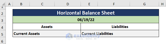
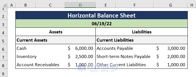
• Then, enter the types of Assets and Liabilities.

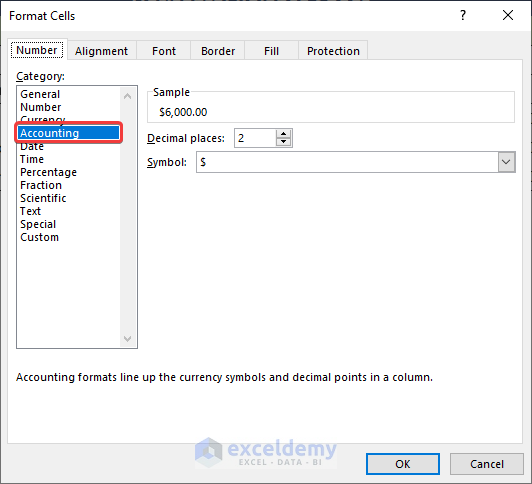
• In general, you should change the number format to Accounting as this is the standard practice when preparing a balance sheet. So, open the Format Cells dialog box by pressing CTRL + 1 and choose Accounting.

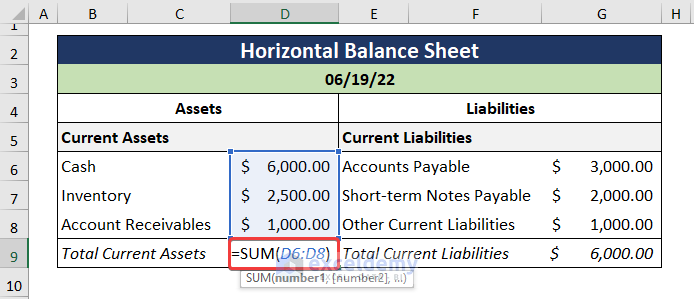
Step 02: Calculate the Assets, Liabilities, and Equities

• Secondly, use the SUM function to compute the sub-total for the Total Current Assets.

In this formula, the D6:D8 cells refer to the Current Assets.

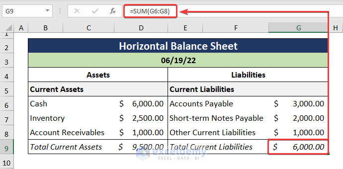
• Likewise, calculate the sum for the Total Current Liabilities.

In the above expression, the G6:G8 cells represent the Current Liabilities.

• Thirdly, we add Fixed Assets and calculate the Total Fixed Asset.

Here, the cells D11:D12 consist of the Fixed Assets.

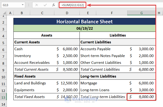
• In a similar fashion, we calculate the Long-term Liabilities.

In this example, the G11:G12 cells represent the Long-term Liabilities.

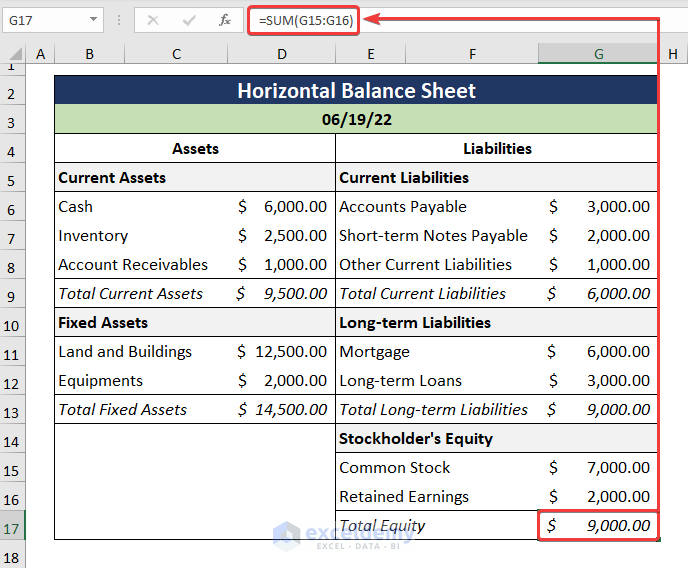
• Now, include the Stockholder’s Equity in the Liabilities column and compute the Total Equity as illustrated below.

Here, the G15:G16 cells consist of the Stockholder’s Equity.

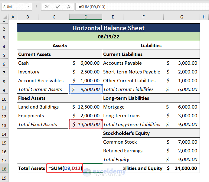
Step 03: Calculate the Total Assets and the Liabilities

• Consequently, we get the Total Assets by adding up the Total Current Assets and Total Fixed Assets.

In this formula, the D9 cell refers to the Total Current Assets while the D13 cell indicates the Total Fixed Assets.

• Moreover, the Total Liabilities and Equity is obtained in the same way.

In the above expression, the G9 cell points to the Total Current Liabilities, next the G13 cell refers to the Total Long-term Liabilities, and finally, the G17 cell indicates the Total Equity.

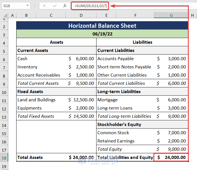
• Considering the general principles of Accounting, the values on both the Total Assets and the Total Liabilities and Equity columns must be equal.

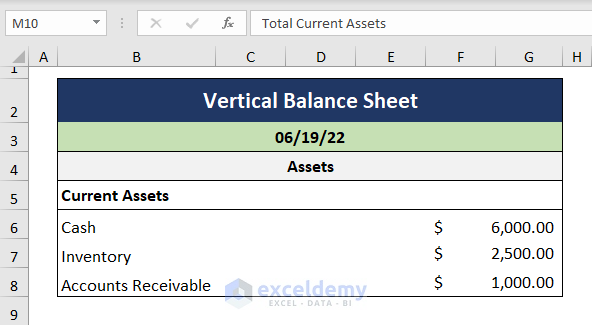
Read More: Balance Sheet Format of a Company in Excel (Download Free Template)

2. Vertical Balance Sheet

A vertical balance sheet consists of two tables one on top of the other. Generally, the Assets column is shown on the top, and the Liabilities and Equities are shown below. Now, to construct a Vertical balance sheet, just follow these steps.

Step 01: Calculate Total Assets

• Firstly, make a heading named Assets followed by a sub-heading for Current Assets.
• Next, enter the Current Asset types on the left side and record the assets’ values on the right side.

• Generally speaking, the Accounting number format is preferable when making balance sheets. So, press CTRL + 1 to open a dialog box and select Accounting.

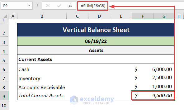
• Following, compute the Total Current Assets using the SUM function.

In this formula, the F6:G8 cells refer to the types of Current Assets.

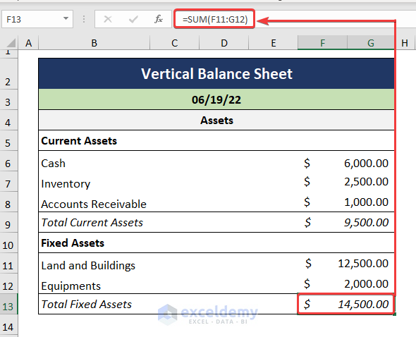
• In turn, compute the Total Fixed Assets as shown below.

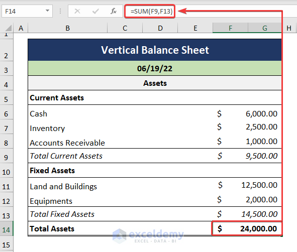
• Eventually, we get the Total Assets by adding up the Fixed Assets and the Current Assets.

In the above formula, the F9 cell indicates the Total Current Assets, and the F13 cell points to the Total Fixed Assets.

Step 02: Compute Total Liabilities

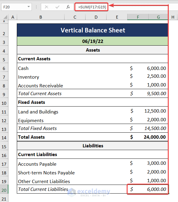
• Secondly, we enter the types and the corresponding values of the Current Liabilities respectively.
• Following, we calculate the Total Current Liabilities as portrayed below.

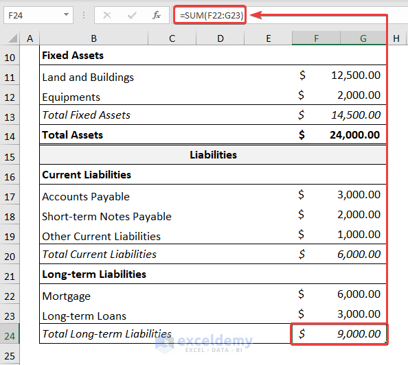
• Then, we calculate the Long-term Liabilities as shown below.

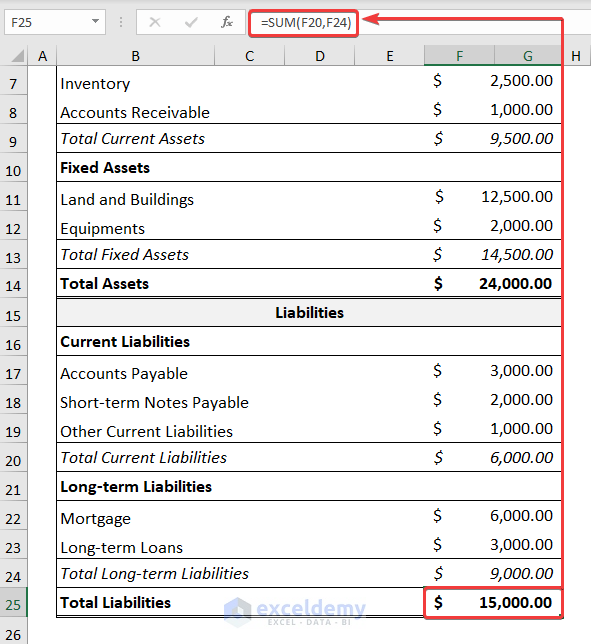
• Hence, the Total Liabilities consist of the summation of Current Liabilities and Long-term Liabilities.

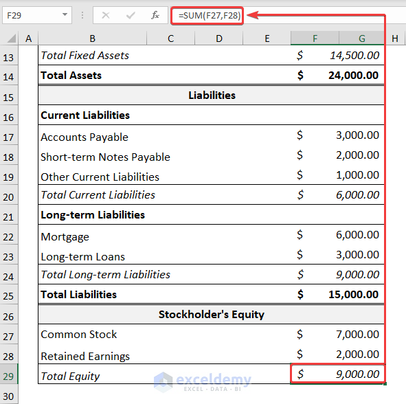
• Last but not the least, we obtain the Total Equity using the same process as before.

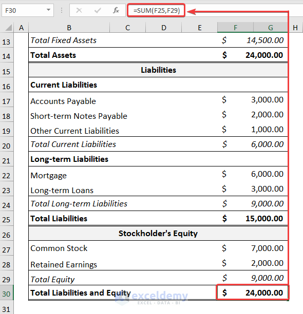
• Finally, we obtain the Total Liabilities and Equity.

In the above expression, the F25 cell points to the Total Liabilities, and the F29 cell indicates the Total Equity.

Read More: Balance Sheet Format in Excel for Proprietorship Business

Conclusion

To conclude, I hope you found in this article what you were looking for. If you have any queries, please leave a comment below. Also, if you want to read more articles like this, you can visit our website ExcelDemy.